Darwin backwards?

What is it with ID proponents and gambling?  Or rather, what is it that makes people who play p0ker and roulette think that that gives them a relevant background for statistical hypothesis testing and an understanding of stochastic processes such as evolution?  Today, “niwrad”, has a post at UD, with one of the most extraordinary garblings of evolutionary theory I think I have yet seen.  He has decided that p0ker is an appropriate model this time (makes a change from coin tossing, I guess).

Continue reading

Randomness and evolution

Here’s a simple experiment one can actually try. Take a bag of M&M’s, and without peeking reach in and grab one. Eat it. Then grab another and return it to the bag with another one, from a separate bag, of the same colour. Give it a shake. I guarantee (and if you tell me how big your bag is I’ll have a bet on how long it’ll take) that your bag will end up containing only one colour. Every time. I can’t tell you which colour it will be, but fixation will happen.
Continue reading

Lizzie asked me a question, so I will respond

Sal Cordova responded to my OP at UD, and I have given his post in full below.

Dr. Liddle recently used my name specifically in a question here:

Chance and 500 coins: a challenge

Barry? Sal? William?

I would always like to stay on good terms with Dr. Liddle. She has shown great hospitality. The reason I don’t visit her website is the acrimony many of the participants have toward me. My absence there has nothing to do with her treatment of me, and in fact, one reason I was ever there in the first place was she was one of the few critics of ID that actually focused on what I said versus assailing me personally.

So, apologies in advance Dr. Liddle if I don’t respond to every question you field. It has nothing to do with you but lots to do with hatred obviously direct toward me by some of the people at your website.

I’ve enjoyed discussion about music and musical instruments.

Continue reading

Proof: Why naturalist science can be no threat to faith in God

I’m going to demonstrate this using Bayes’ Rule. I will represent the hypothesis that (a non-Deist, i.e. an interventionist) God exists as H_G, and the evidence of complex life as L_C.  What we want to know is the posterior probability that H_{G} is true, given L_C, written

    \[P(H_{G}|L_N)}\]

which, in English, is: the probability that God exists, given the evidence before us of complex life.

Continue reading

Chance and 500 coins: a challenge

My problem with the IDists’ 500 coins question (if you saw 500 coins lying heads up, would you reject the hypothesis that they were fair coins, and had been fairly tossed?)  is not that there is anything wrong with concluding that they were not.  Indeed, faced with just 50 coins lying heads up, I’d reject that hypothesis with a great deal of confidence.

It’s the inference from that answer of mine is that if, as a “Darwinist” I am prepared to accept that a pattern can be indicative of something other than “chance” (exemplified by a fairly tossed fair coin) then I must logically also sign on to the idea that an Intelligent Agent (as the alternative to “Chance”) must inferrable from such a pattern.

This, I suggest, is profoundly fallacious.

Continue reading

Barry gets it wrong again….

Here.


The null hypothesis in a drug trial is not that the drug is efficacious. The null hypothesis is that the difference between the groups is due to chance.

No, Barry.  Check any stats text book.  The null hypothesis is certainly not that the drug is efficacious (which is not what Neil said), but more importantly, it is not that “the difference between the groups is due to chance”.

It is that “there is no difference in effects between treatment A and treatment B”.

When in hole, stop digging, Barry!

Continue reading

Yes, Lizzie, Chance is Very Often an Explanation

[Posted by Barry at UD]

Over at The Skeptical Zone Elizabeth Liddle has weighed in on the “coins on the table” issue I raised in this post.

Readers will remember the simple question I asked:

If you came across a table on which was set 500 coins (no tossing involved) and all 500 coins displayed the “heads” side of the coin, how on earth would you test “chance” as a hypothesis to explain this particular configuration of coins on a table?

Dr. Liddle’s answer:

Chance is not an explanation, and therefore cannot be rejected, or supported, as a hypothesis.

Staggering. Gobsmacking. Astounding. Superlatives fail me.

Continue reading

Getting from Fisher to Bayes

(slightly edited version of a comment I made at UD)

Barry Arrington has  a rather extraordinary thread at UD right now, ar

Jerad’s DDS Causes Him to Succumb to “Miller’s Mendacity” and Other Errors

It arose from a Sal’s post, here at TSZ, Siding with Mathgrrl on a point,and offering an alternative to CSI v2.0

Below is what I posted in the UD thread.

Continue reading

Siding with Mathgrrl on a point,and offering an alternative to CSI v2.0

[cross posted from UD Siding with Mathgrrl on a point, and offering an alternative to CSI v2.0, special thanks to Dr. Liddle for her generous invitation to cross post]

There are two versions of the metric for Bill Dembski’s CSI. One version can be traced to his book No Free Lunch published in 2002. Let us call that “CSI v1.0”.

Then in 2005 Bill published Specification the Pattern that Signifies Intelligence where he includes the identifier “v1.22”, but perhaps it would be better to call the concepts in that paper CSI v2.0 since, like windows 8, it has some radical differences from its predecessor and will come up with different results. Some end users of the concept of CSI prefer CSI v1.0 over v2.0.
Continue reading

Specification for Dummies

I’m lookin’ at you, IDers 😉

Dembski’s paper: Specification: The Pattern That Specifies Complexity gives a clear definition of CSI.

The complexity of pattern (any pattern) is defined in terms of Shannon Complexity.  This is pretty easy to calculate, as it is merely the probability of getting this particular pattern if you were to randomly draw each piece of the pattern from a jumbled bag of pieces, where the bag contains pieces in the same proportion as your pattern, and stick them together any old where.  Let’s say all our patterns are 2×2 arrangements of black or white pixels. Clearly if the pattern consists of just four black or white pixels, two black and two white* , there are only 16 patterns we can make:

Patterns1And we can calculate this by saying: for each pixel we have 2 choices, black or white, so the total number of possible patterns is 2*2*2*2, i.e 24  i.e. 16. That means that if we just made patterns at random we’d have a 1/16 chance of getting any one particular pattern, which in decimals is .0625, or 6.25%.  We could also be fancy and express that as the negative log 2 of .625, which would be 4 bits.  But it all means the same thing.  The neat thing about logs is that you can add them, and get the answer you would have got if you’d multipled the unlogged numbers.  And as the negative log of .5 is 1, each pixel, for which we have a 50% chance of being black or white, is worth “1 bit”, and four pixels will be worth 4 bits.

Continue reading

Protein Space and Hoyle’s Fallacy – a response to vjtorley

‘vjtorley’ has honoured me with my very own OP at Uncommon Descent in response to my piece on Protein Space. I cannot, of course, respond over there (being so darned uncivil and all!), so I will put my response in this here bottle and hope that a favourable wind will drive it to vjt’s shores. It’s a bit long (and I’m sure not any the better for it…but I’m responding to vjt and his several sources … ! ;)).


“Build me a protein – no guidance allowed!”

The title is an apparent demand for a ‘proof of concept’, but it is beyond intelligence too at the moment, despite a working system we can reverse engineer (a luxury not available to Ye Olde Designer). Of course I haven’t solved the problem, which is why I haven’t dusted off a space on my piano for that Nobel Prize. But endless repetition of Hoyle’s Fallacy from multiple sources does not stop it being a fallacious argument.

Dr Torley bookends his post with a bit of misdirection. We get pictures of, respectively, a modern protein and a modern ribozyme. It has never been disputed that modern proteins and ribozymes are complex, and almost certainly not achievable in a single step. But

1) Is modern complexity relevant to abiogenesis?

2) Is modern complexity relevant to evolution?


Here are three more complex objects:

DESCRIPTION HERE

Circuit Board

DESCRIPTION HERE

Panda playing the flute

DESCRIPTION HERE

er … not yet in service!


Continue reading

Prizegiving!

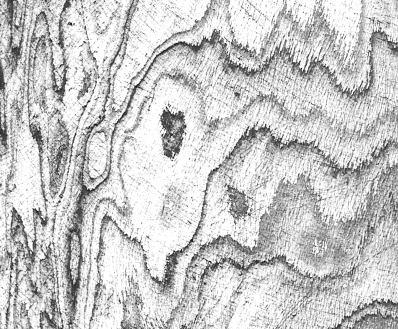
Phinehas and Kairosfocus share second prize for my CSI challenge: yes, it is indeed “Ash on Ice” – it’s a Google Earth image of Skeiðarárjökull Glacier.

But of course the challenge was not to identify the picture, but to calculate its CSI. Vjtorley deserves, I think, first prize, not for calculating it, but for making so clear why we cannot calculate CSI for a pattern unless we can calculate “p(T|H)” for all possible “chance” (where “chance” means “non-design”) hypotheses.

In other words, unless we know, in advance, how likely we are to observe the candidate pattern, given non-chance, we cannot infer Design using CSI. Which is, by the Rules of Right Reason, the same as saying that in order to infer Design using CSI, we must first  calculate how likely our candidate pattern is under all possible non-Design hypotheses.

As Dr Torley rightly says:

Professor Felsenstein is quite correct in claiming that “CSI is not … something you could assess independently of knowing the processes that produced the pattern.”

And also, of course, in observing that Dembski acknowledges this in his paper, , Specification: The Pattern That Signifies Intelligence, as many of us have pointed out.  Which is why we keep saying that it can’t be calculated – you have to be able to quantify p(T|H), where H is the actual non-design hypothesis, not some random-independent-draw hypothesis.

Continue reading

Journal club – Protein Space. Big, isn’t it?

Simplistic combinatorial analyses are an honoured tradition in anti-evolutionary circles. Hoyle’s is the archetype of the combinatorial approach, and he gets a whole fallacy named after him for his trouble. The approach will be familiar – a string of length n composed of v different kinds of subunit is one point in a permutation space containing vn points in total. The chance of hitting any given sequence in one step, such as the one you have selected as ‘target’, is the reciprocal of that number. Exponentiation being the powerful tool it is, it takes only a little work with a calculator to assess the permutations available to the biological polymers DNA and protein and come up with some implausibly large numbers and conclude that Life – and, if you are feeling bold, evolution – is impossible.

Dryden, Thomson and White of Edinburgh University’s Chemistry department argue in this 2008 paper that not only is the combinatorial space of the canonical 20 L-acids much smaller than simplistically assumed, but more surprisingly, that it is sufficiently small to have been explored completely during the history of life on earth. Continue reading

Some Help for IDists: Benford’s Law

Guys, as your scientific output is lacking at the moment, allow me to point you towards Benford’s law: http://en.wikipedia.org/wiki/Benford’s_law

Benford’s law, also called the first-digit law, refers to the frequency distribution of digits in many (but not all) real-life sources of data. In this distribution, the number 1 occurs as the first digit about 30% of the time, while larger numbers occur in that position less frequently: 9 as the first digit less than 5% of the time. This distribution of first digits is the same as the widths of gridlines on a logarithmic scale. Benford’s law also concerns the expected distribution for digits beyond the first, which approach a uniform distribution.


TSZ team: Can we build this into a statistically testable (Null hypothesis?) ID Hypothesis?

This one piqued my interest:

“Frequency of first significant digit of physical constants plotted against Benford’s law” – Wikipedia

Is evolution of proteins impossible?

At Uncommon Descent, “niwrad” has posted a link to a Sequences Probability Calculator. This webserver allows you to set a number of trials (“chemical reactions”) per second, the number of letters per position (20 for amino acids) and a sequence length, and then it calculates how long it will take for you to get exactly that sequence. Each trial assumes that you draw a sequence at random, and success is only when you exactly match the target sequence. This of course takes nearly forever.

So in effect the process is one of random mutation without natural selection present, or random mutation with natural selection that shows no increase in fitness when a sequence partially matches the target. This leads to many thoughts about evolution, such as:

  • Do different species show different sequences for a given protein? Typically they do, so the above scheme implies that they can’t have evolved from common ancestors that had a different protein sequence. They each must have been the result of a separate special creation event.
  • If an experimenter takes a gene from one species and puts it into another, so that the protein sequence is now that of the source species, does it still function? If not, why are people so concerned about making transgenic organisms (they’d all be dead anyway)?
  • If we make a protein sequence by combining part of a sequence from one species and the rest of that protein sequence from another, will that show function in either of the parent species? (Typically yes, it will).

Does a consideration of the experimental evidence show that the SPC fails to take account of the function of nearby sequences?

The author of the Sequences Probability Calculator views evolution as basically impossible. The SPC assumes that any change in a protein makes it unable to function. Each species sits on a high fitness peak with no shoulders. In fact, experimental studies of protein function are usually frustrating, because it is hard to find noticeable difference of function, at least ones big enough to measure in the laboratory.

The LCI and Bernoulli’s Principle of Insufficent Reason

(Just found I can post here – I hope it is not a mistake. This is a slightly shortened version of a piece which I have published on my blog. I am sorry it is so long but I struggle to make it any shorter. I am grateful for any comments. I will look at UD for comments as well – but not sure where they would appear.).

I have been rereading Bernoulli’s Principle of Insufficient Reason and Conservation of Information in Computer Search by William Dembski and Robert Marks. It is an important paper for the Intelligent Design movement as Dembski and Marks make liberal use of Bernouilli’s Principle of Insufficient Reason (BPoIR) in their papers on the Law of Conservation of Information (LCI).  For Dembski and Marks BPoIR provides a way of determining the probability of an outcome given no prior knowledge. This is vital to the case for the LCI.

The point of Dembski and Marks paper is to address some fundamental criticisms of BPoIR. For example  J M Keynes (along with with many others) pointed out that the BPoIR does not give a unique result. A well-known example is applying BPoIR to the specific volume of a given substance. If we know nothing about the specific volume then someone could argue using BPoIR that all specific volumes are equally likely. But equally someone could argue using BPoIR all specific densities are equally likely. However, as one is the reciprocal of the other, these two assumptions are incompatible. This is an example based on continuous measurements and Dembski and Marks refer to it in the paper. However, having referred to it, they do not address it. Instead they concentrate on the examples of discrete measurements where they offer a sort of response to Keynes’ objections. What they attempt to prove is a rather limited point about discrete cases such as a pack of cards or protein of a given length. It is hard to write their claim concisely – but I will give it a try.

Imagine you have a search space such as a normal pack of cards and a target such as finding a card which is a spade. Then it is possible to argue by BpoIR that, because all cards are equal, the probability of finding the target with one draw is 0.25. Dembski and Marks attempt to prove that in cases like this that if you decide to do a “some to many” mapping from this search space into another space then you have at best a 50% chance of creating a new search space where BPoIR gives a higher probability of finding a spade. A “some to many” mapping means some different way of viewing the pack of cards so that it is not necessary that all of them are considered and some of them may be considered more often than others. For example, you might take a handful out of the pack at random and then duplicate some of that handful a few times – and then select from what you have created.

There are two problems with this.

1) It does not address Keynes’ objection to BPoIR

2) The proof itself depends on an unjustified use of BPoIR.

But before that a comment on the concept of no prior knowledge.

The Concept of No Prior Knowledge

Dembski and Marks’ case is that BPoIR gives the probability of an outcome when we have no prior knowledge. They stress that this means no prior knowledge of any kind and that it is “easy to take for granted things we have no right to take for granted”.  However, there are deep problems associated with this concept. The act of defining a search space and a target implies prior knowledge. Consider finding a spade in pack of cards. To apply BPoIR at minimum you need to know that a card can be one of four suits, that 25% of the cards have a suit of spades, and that the suit does not affect the chances of that card being selected. The last point is particularly important. BPoIR provides a rationale for claiming that the probability of two or more events are the same. But the events must differ in some respects (even if it is only a difference in when or where they happen) or they would be the same event. To apply BPoIR we have to know (or assume) that these differences are not relevant to the probability of the events happening. We must somehow judge that the suit of the card, the head or tails symbols on the coin, or the choice of DNA base pair is irrelevant to the chances of that card, coin toss or base pair being selected. This is prior knowledge.

In addition the more we try to dispense with assumptions and knowledge about an event then the more difficult it becomes to decide how to apply BPoIR. Another of Keynes’ examples is a bag of 100 black and white balls in an unknown ratio of black to white. Do we assume that all ratios of black to white are equally likely or do we assume that each individual ball is equally likely to be black or white? Either assumption is equally justified by BPoIR but they are incompatible. One results in a uniform probability distribution for the number of white balls from zero to 100; the other results in a binomial distribution which greatly favours roughly equal numbers of black and while balls.

Looking at the problems with the proof in Dembski and Marks’ paper.

The Proof does not Address Keynes’ objection to BPoIR

Even if the proof were valid then it does nothing to show that the assumption of BPoIR is correct. All it would show (if correct) was that if you do not use BPoIR then you have 50% or less chance of improving your chances of finding the target. The fact remains that there are many other assumptions you could make and some of them greatly increase your chances of finding the target. There is nothing in the proof that in anyway justifies assuming BPoIR or giving it any kind of privileged position.

But the problem is even deeper. Keynes’ point was not that there are alternatives to using BPoIR – that’s obvious. His point was that there are different incompatible ways of applying BPoIR. For example, just as with the example of black and white balls above, we might use BPoIR to deduce that all ratios of base pairs in a string of DNA are equally likely. Dembski and Marks do not address this at all. They point out the trap of taking things for granted but fall foul of it themselves.

The Proof Relies on an Unjustified Use of BPoIR

The proof is found in appendix A of the paper and this is the vital line:

image

This is the probability that a new search space created from an old one will include k members which were part of the target in the original search space. The equation holds true if the new search space is created by selecting elements from old search space at random; for example, by picking a random number of cards at random from a pack. It uses BPoIR to justify the assumption that each unique way of picking cards is equally likely. This can be made clearer with an example.

Suppose the original search space comprises just the four DNA bases, one of which is the target. Call them x, y, z and t. Using BPoIR, Dembski and Marks would argue that all of them are equally likely and therefore the probability of finding t with a single search is 0.25. They then consider all the possible ways you might take a subset of that search space. This comprises:

Subsets with

no items

just one item: x,y,z and t

with two items: xy, xz, yz, tx, ty, tz

with three items: xyz, xyt, xzt, yzt

with four items: xyzt

A total of 16 subsets.

Their point is that if you assume each of these subsets is equally likely (so the probability of one of them being selected is 1/16) then 50% of them have a probability of finding t which is greater than or equal to probability in the original search space (i.e. 0.25). To be specific new search spaces where probability of finding t is greater than 0.25 are t, tx, ty, tz, xyt, xzt, yzt and xyzt. That is 8 out of 16 which is 50%.

But what is the justification for assuming each of these subsets are equally likely? Well it requires using BPoIR which the proof is meant to defend. And even if you grant the use of BPoIR Keynes’ concerns apply. There is more than one way to apply BPoIR and not all of them support Dembski and Marks’ proof. Suppose for example the subset was created by the following procedure:

    • Start with one member selected at random as the subset
    • Toss a dice,
      • If it is two or less then stop and use current set as subset
      • If it is a higher than two then add another member selected at random to the subset
    • Continue tossing until dice throw is two or less or all four members in are in subset

This gives a completely different probability distribution.

The probability of:

single item subset (x,y,z, or t) = 0.33/4 = 0.083

double item subset (xy, xz, yz, tx, ty, or tz) = 0.66*0.33/6 = 0.037

triple item subset (xyz, xyt, xzt, or yzt) = 0.66*0.33*0.33/4 = 0.037

four item subset (xyzt) = 0.296

So the combined probability of the subsets where probability of selecting t is ≥ 0.25 (t, tx, ty, tz, xyt, xzt, yzt, xyzt) = 0.083+3*(0.037)+3*(0.037)+0.296 = 0.60 (to 2 dec places) which is bigger than 0.5 as calculated using Dembski and Marks assumptions. In fact using this method, the probability of getting a subset where the probability of selecting t ≥ 0.25 can be made as close to 1 as desired by increasing the probability of adding a member. All of these methods treat all four members of the set equally and are equally justified under BpoIR as Dembski and Marks assumption.

Conclusion

Dembski and Marks paper places great stress on BPoIR being the way to calculate probabilities when there is no prior knowledge. But their proof itself includes prior knowledge. It is doubtful whether it makes sense to eliminate all prior knowledge, but if you attempt to eliminate as much prior knowledge as possible, as Keynes does, then BPoIR proves to be an illusion. It does not give a unique result and some of the results are incompatible with their proof.