
I’m lookin’ at you, IDers 😉
Dembski’s paper: Specification: The Pattern That Specifies Complexity gives a clear definition of CSI.
The complexity of pattern (any pattern) is defined in terms of Shannon Complexity. This is pretty easy to calculate, as it is merely the probability of getting this particular pattern if you were to randomly draw each piece of the pattern from a jumbled bag of pieces, where the bag contains pieces in the same proportion as your pattern, and stick them together any old where. Let’s say all our patterns are 2×2 arrangements of black or white pixels. Clearly if the pattern consists of just four black or white pixels, two black and two white* , there are only 16 patterns we can make:
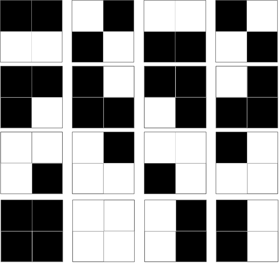 And we can calculate this by saying: for each pixel we have 2 choices, black or white, so the total number of possible patterns is 2*2*2*2, i.e 24 i.e. 16. That means that if we just made patterns at random we’d have a 1/16 chance of getting any one particular pattern, which in decimals is .0625, or 6.25%. We could also be fancy and express that as the negative log 2 of .625, which would be 4 bits. But it all means the same thing. The neat thing about logs is that you can add them, and get the answer you would have got if you’d multipled the unlogged numbers. And as the negative log of .5 is 1, each pixel, for which we have a 50% chance of being black or white, is worth “1 bit”, and four pixels will be worth 4 bits.
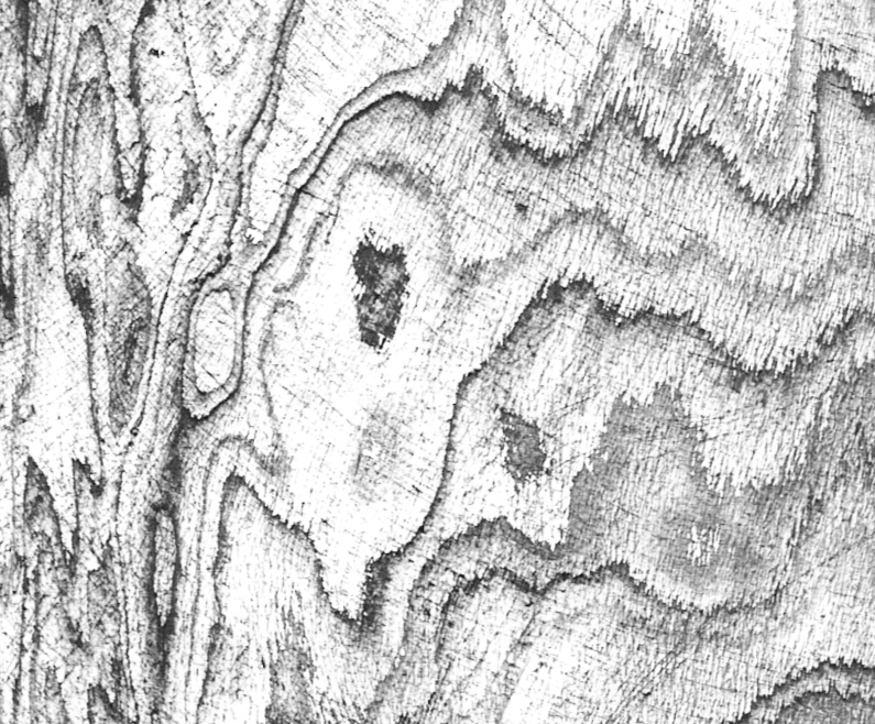
So if we go back to my nice greyscale image of Skeiðarárjökull Glacier, we can easily calculate its complexity in bits. There are 256 possible colours for each pixel, and there are 658 x 795 pixels in the image, i.e 523,110 pixels. If all the colours were equally represented, there would be 8 bits per pixel (because the negative log 2 of 1/256 is 8), and we’d have 8*658 *795 bits, which is about 4 million bits. In fact it’s a bit less than that, because not all colours are equally represented (light pixels are more common than dark) but it’s still very large. So we can say that my pattern is complex by Dembski’s definition. (The fact that it’s a photo of the glacier is irrelevant – the photo is just a simplified version of the original pattern, with a lot of the detail – the information – of the original removed. So if my picture has specified complexity, the glacier itself certainly will).
But the clever part of Dembski’s idea is the idea of Specification. He proposes that we define a specification by the descriptive complexity of the pattern – the more simply it can be described, the more specified it is. So “100 heads” for 100 coin tosses is far simpler to describe than “HHTTHHTHHTHTHHTHTHTHTHHTTHTTTTTH….” and all the other complicated patterns that you might toss. So if we tossed 100 heads, we’d be very surprised, and smell a rat, even though the pattern is actually no less likely any other single pattern that we could conceivably toss. And so Dembski says that if our “Target” or candidate pattern is part of a subset of possible patterns that can be described as, or more simply, than the Target pattern it is Specified, and if that subset is a very small proportion of the whole range of possible patterns, we can say it is Specified and Complex (because very low probability on a single draw, therefore lots of bits).
When I chose my glacier pattern I chose it because it is quite distinctive. It features waving bands of dark alternating with light. One way we can describe such a pattern is in terms of its “autocorrelation” – how well the value of one pixel predicts the value of the next. If the pattern consisted of perfectly graded horizontal bands of grey, shaded from dark at the top to light at the bottom, the autocorrelation would be near 1 (near, because it wouldn’t necessarily be exactly linear). And so we could write a very simple equation that described the colour of each pixel, with a short accompanying list of pixels that didn’t quite equal the value predicted by the equation.
However, for the vast majority of patterns drawn from that pool of pixel colours, you’d pretty well need to describe every pixel separately (which is why bitmaps take so much memory).
So one very easy way of figuring out how the “descriptive complexity” (or simplicity, rather) of my pattern was to compute the mean autocorrelation across all the columns and rows of my image. And it was very high. The correlation value was .89 which is a very high correlation – not surprisingly as the colours are very strongly clustered. And so I know that the simplest possible description of my pattern is going to be a lot simpler than for a randomly drawn pattern of pixels.
To calculate what proportion of randomly drawn patterns would have this high a mean autocorrelation, I ran a Monte Carlo simulation (with 10,000 iterations) so that I could estimate the mean autocorrelation of randomly drawn patterns, and the standard deviation of those correlations (for math nitpickers I first Fisher transformed the correlations, to normalise the distribution, as one should). That gave me my distribution of autocorrelations under the null of random draws. And I found, as I expected, that the mean was near zero, and the standard deviation very small. And having got that standard deviation, I was able to work out how many standard deviations my image correlation was from the mean of the random image.
The answer was over 4000. Now, we can convert that number of standard devions to a probability – the probability of getting that pattern from random draws. And it is so terribly tiny, that my computer just coughed up “inf”. However, that’s OK, because it could cope with telling me how many standard deviations it would have to be to be less than Dembski’s threshold of 1/1*150, which is only 26 standard deviations. So we know it is way way way way under the the Bound (or, if you want to express the Bound in bits, way way way way way over 500 bits).
So, by Dembski’s definition, my pattern is Complex (has lots of Shannon Bits). Moreoever, by Dembski’s definition, my pattern is Specified (it can be described much more simply than most random patterns). And when we compute that Specified Complexity in Bits, by figuring out what proportion of possible patterns the patterns that can be described as or more simply than my pattern, it is way way way way way way more than 500 bits.
So, can we infer Design, by Dembski’s definition?
No, because Dembski has a third hurdle that my pattern has to vault, one that for some reason the Uncommon Descenters keep forgetting (with some commendable exceptions, I’m looking at you, Dr Torley :))
What that vast 500 bit plus number represents (my 4000+ standard deviations) is the probability that I would produce that pattern, or one with as high a mean autocorrelation, if I kept on running my Monte Carlo simulation for the lifetime of the Universe. In other words, it’s the probability of my pattern, given only random independent draws from my pool of pixels: p(T|H) where H is random independent draws. But that’s not what Dembski says H is. (Kairosfocus, you should have spotted this, but you didn’t).
Dembski says that H is “the relevant chance hypothesis” (my bold), “taking into account Darwinian and other material mechanisms“. Well, for a card dealer, or a coin-tosser, the “relevant chance hypothesis” is indeed “random independent draws”. But we aren’t talking about that “chance” hypothesis here (for Dembski, “chance” appears to mean “non-design, i.e. he collapses Chance and Necessity from his earlier Explanatory Filter). So we need to compute not just p(T|H) where H is random independent draws: we need to compute p(T|H) where H is the relevant chance hypothesis.
Now, because Phinehas and Kairosfocus both googled my pattern and, amazingly, found it (google is awesome) they had a far better chance of computing p(T|H) reasonably, because they could form a “relevant chance [non-design] hypothesis”. Well, I say “compute” but “have a stab at” is probably a better term. Once they knew it was ash on a glacier, they could ask: what is the probability of a pattern like Lizzie’s, given what we know about the patterns volcanic ash forms on glaciers? Well, we know that it forms patterns just like mine, because they actually found it doing just that! Therefore p(T|H) is near 1, and its the number of Specified Complexity bits near zero, not Unfeasibly Vast.
But, Kairosfocus, before you go and enjoy your success, consider this:
- Firstly: if you had computed the CSI without knowing what the picture was of, you would have been stumped: without knowing what it was, there is no way of computing p(T|H) and if you had used random independent draws as a default, you would have got a false positive for Design.
- Secondly: You got the right answer but gave the wrong reason. You and Eric Anderson both thought that CSI (or the EF) had yielded a correct negative because my pattern wasn’t Specified. It is. Its specification is exactly as Dembski described it. The reason you concluded it was not designed was because you didn’t actually compute CSI at all. What you needed to do was to compute p(T|H). But you could only do that if you knew what the thing was in the first place, figured out how it had been made, and that it was the result of “material mechanisms”! In other words, CSI will only give you the answer if you have some way of computing the p(T|H) where H is the relevant chance hypothesis.
And, as Dr Torley rightly says, you can only do that if you know what the thing is and how it was, or might have been, produced by any non-design mechanisms. And not only that, you’ve got to be able to compute the probability of getting the pattern by those mechanisms, including the ones you haven’t thought of!
So: how do you compute CSI for a pattern where the relevant chance [non-design] hypothesis is not simply “independent random draws”?
I suggest it is impossible. I suggest moreover, that Dembski is, even within that paper, completely contradicting himself. In that same paper, where he says that we must take into account “Darwinian and other mechanisms” when computing p(T|H), he also says:
By contrast, to employ specified complexity to infer design is to take the view that objects, even if nothing is known about how they arose, can exhibit features that reliably signalthe action of an intelligent cause.
If we know nothing about how they arose (as was the case before KF and Phinehas googled it) you would have no basis on which to calculate p(T|H), unless you assumed random independent draws, which would, as we have seen, give you a massively false positive. You can get the right answer if you do know something about how it arose, but then CSI isn’t doing the job it is supposed to.
Conclusion:
CSI can’t be computed, unless you know the answer before you compute it.
* h/t to cubist. I changed my scenario mid-composition, but forgot to change this text!
I think Axe attempts to address some of the issues here: The Case Against a Darwinian Origin of Protein Folds in Bio-Complexity, but I haven’t read it. Has anyone?
Some pdf text didn’t copy correctly, particularly in the math, so beware.