Prof. Marks gets lucky at Cracker Barrel

Posted on January 18, 2018 by DiEb

Introduction to Evolutionary Informatics, by Robert J. Marks II, the “Charles Darwin of Intelligent Design”; William A. Dembski, the “Isaac Newton of Information Theory”; and Winston Ewert, the “Charles Ingram of Active Information.” World Scientific, 332 pages.

Classification: Engineering mathematics. Engineering analysis. (TA347)
Subjects: Evolutionary computation. Information technology–Mathematics.

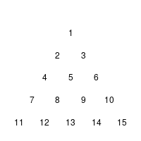
Yesterday, I looked again through “Introduction to Evolutionary Informatics”, when I spotted the Cracker Barrel puzzle in section 5.4.1.2 Endogenous information of the Cracker Barrel puzzle (p. 128). The rules of this variant of a triangular peg-solitaire are described in the text (or can be found at wikipedia’s article on the subject).

The humble authors¹ then describe a simulation of the game to calculate how probable it is to solve the puzzle using moves at random:

A search typically requires initialization. For the Cracker Barrel puzzle, all of the 15 holes are filled with pegs and, at random, a single peg is removed. This starts the game. Using random initialization and random moves, simulation of four million games using a computer program resulted in an estimated win probability p = 0.0070 and an endogenous information of

$I_\Omega = -\log_2 p = 7.15 bits.$

Winning the puzzle using random moves with a randomly chosen initialization (the choice of the empty hole at the start of the game) is thus a bit more difficult than flipping a coin seven times and getting seven heads in a row

Naturally, I created such an simulation in R for myself: I encoded all thirty-six moves that could occur in a matrix cb.moves, each row indicating the jumping peck, the peck which is jumped over, and the place on which the peck lands.

And here is the little function which simulates a single random game:

cb.simul <- function(pos){
# pos: boolean vector of length 15 indicating position of pecks # a move is allowed if there is a peck at the start position & on the field which is # jumped over, but not at the final position allowed.moves <- pos[cb.moves[,1]] & pos[cb.moves[,2]] & (!pos[cb.moves[,3]]) # if no move is allowed, return number of pecks left if(sum(allowed.moves)==0) return(sum(pos)) # otherwise, choose an allowed move at random number.of.move <- ((1:36)[allowed.moves])[sample(1:sum(allowed.moves),1)] pos[cb.moves[number.of.move,]] <- c(FALSE,FALSE,TRUE) return(cb.simul(pos)) }

I run the simulation 4,000,000 times, changing the start position at random. But as a result, my estimated win probability was $p_e=0.0045$ – only two thirds of the number in the text. How could this be? Why were Prof. Marks et.al. so much luckier than I? I re-run the simulation, checked the code, washed, rinsed, repeated: no fundamental change.

So, I decided to take a look at all possible games and on the probability with which they occur. The result was this little routine:

cb.eval <- function(pos, prob){
#pos: boolean vector of length 15 indicating position of pecks #prob: the probability with which this state occurs # a move is allowed if there is a peck at the start position & on the field which is #jumped over, but not at the final position allowed.moves <- pos[cb.moves[,1]] & pos[cb.moves[,2]] & (!pos[cb.moves[,3]]) if(sum(allowed.moves)==0){ #end of a game: prob now holds the probability that this game is played nr.of.pecks <- sum(pos) #number of remaining pecks cb.number[nr.of.pecks] <<- cb.number[nr.of.pecks]+1 #the number of remaining pecks is stored in a global variable cb.prob[nr.of.pecks] <<- cb.prob[nr.of.pecks] + prob #the probability of this game is added to the appropriate place of the global variable return() } for(k in 1:sum(allowed.moves)){ #moves are still possible, for each move the next stage will be calculated d <- pos number.of.move <- ((1:36)[allowed.moves])[k] d[cb.moves[number.of.move,]] <- c(FALSE,FALSE,TRUE) cb.eval(d,prob/sum(allowed.moves)) } }

I now calculated the probabilities for solving the puzzle for each of the fifteen possible starting positions. The result was

$p_s=0.0045 .$

This fits my simulation, but not the one of our esteemed and humble authors! What had happened?

An educated guess

I found it odd that the authors run 4,000,000 simulations – 1,000,000 or 10,000,000 seem to be more commonly used numbers. But when you look at the puzzle, you see that it was not necessary for me to look at all fifteen possible starting positions – whether the first peck is missing in position 1 or position 11 does not change the quality of the game: you could rotate the board and perform the same moves. Using symmetries, you find that there are only four essentially different starting positions. the black, red, and blue group with three positions each, and the green group with six positions. For each group, you get a different probability of success

group	black	green	red	blue
prob. of choosing this group	.2	.4	.2	.2
prob. of success	.00686	.00343	.00709	.001726

One quite obvious explanation for the result of the authors is that they did not run one simulation using a random starting position for 4,000,000 times, but simulated for each of the four groups the game 1,000,000 times. Unfortunately they either did not cumulate their results, but took only the one of the results of the black or the red group (or both), or they only thought they switched starting positions from one group of simulations to the next, but indeed always used the black or the red one.

Is it a big deal?

It is easily corrigible: instead of “For the Cracker Barrel puzzle, all of the 15 holes are filled with pegs and, at random, a single peg is removed.” they could write “For the Cracker Barrel puzzle, all of the 15 holes are filled with pegs and, one peck at the tip of the triangle is removed.”

If the book was actually used as a textbook, the simulation of the Cracker Barrel puzzle is an obvious exercise. I doubt that it is used that way anywhere, so no pupils were annoyed.

It is somewhat surprising that such an error occurs: it seems that the program was written by a single contributor and not checked. That seems to have been the case in previous publications, too.

Perhaps the authors thought that the program was too simple to be worthy of their full attention – and the more complicated stuff is properly vetted. OTOH, it could be a pattern….

Well, it will certainly be changed in the next edition.

(Cross-posted from here)

^{1. p.13, 118, 142, and 173↩}

54 thoughts on “Prof. Marks gets lucky at Cracker Barrel”

Corneel on January 18, 2018 at 4:39 pm said:

I tried to rapidly run your code in R, but I note I need to create the cb.moves object first. That will be a nice project for the weekend.

How long did it take to run the simulations?
Alan Fox on January 18, 2018 at 5:04 pm said:

Welcome back DiEb. Hope you are keeping well. I’m sure most members recall DiEb’s fascinating analyses comparing activity at TSZ and Uncommon Descent.

I’m crossing fingers that DiEb might find time to post something for 2017.

*crosses fingers and wishes*
DiEb on January 18, 2018 at 5:48 pm said:

Corneel:
I tried to rapidly run your code in R, but I note I need to create the cb.moves object first. That will be a nice project for the weekend.

How long did it take to run the simulations?

An independent developed verification/falsification would be lovely!

The simulations run quickly, the longest were the 4,000,000 simulations which took a few minutes.
keiths on January 18, 2018 at 9:31 pm said:

DiEb:

It is somewhat surprising that such an error occurs: it seems that the program was written by a single contributor and not checked. That seems to have been the case in previous publications, too.

I get the same impression. We examined one of their papers here:

Algorithmic Specified Complexity and the Game of Life

In that thread we identified well over 20(!) substantive errors in the paper. Either the co-authors didn’t check each others’ work, or they are all extremely incompetent.
Tom English on January 19, 2018 at 2:47 am said:

Good to see you, DiEb.

I don’t have many neurons firing at the moment. But I’m thinking (to put it generously) that dynamic programming would work nicely here. The number of paths (from initial states) to a state is

(a) 1 if the state is an initial state, i.e., with just one empty hole, and
(b) the sum of the numbers of paths to the immediate predecessors of the state, otherwise.

There may be a trick for stopping the recursion at 7 pegs, because playing the game backward (filling jumped holes), is essentially the same as playing the game forward (emptying jumped holes). The state space is not large, but I’m curious, anyway, as to whether the forward-backward symmetry is exploitable.

The number of paths from initial states to goal states (with exactly one peg) divided by the number of paths from initial states to terminal states (with no successor states) is the number we’re looking for — right?
DiEb on January 19, 2018 at 8:43 am said:

Tom English,

Nice to see you, too!
1) The space is rather small, according to my calculations, there are only 7,335,390 possible games using all of the fifteen different starting positions.
2) 438,984 of these games are successful with only one peck left standing, that’s 5.984% of the games
3) Here’s the rub: not all games are equally likely to happen. The chance to play a perfect game at random is just 0.451% !
4) The more successful an individual game is, the more decisions have to be made, the less probable it becomes: there are only six games which will leave you with a frustrating number of 10 pecks still standing, but the chance that such a game occurs at random is 0.444% – only little less than a perfect game.
5) On average, you will end up with four pecks – and that is the most probable outcome, too – 47.8%
Tom English on January 19, 2018 at 9:08 am said:

DiEb: Here’s the rub: not all games are equally likely to happen

I hope I haven’t misunderstood. All I have left to do, to get some data, is to set up the operators. However, that’s tedious and error-prone, and I may put it aside until tomorrow.

Thanks for the data. The probability distribution over the numbers of pecks at the end of the game would be handy. [ETA: But knowing several key probabilities is fine.]
Tom English on January 19, 2018 at 2:40 pm said:

DiEb: 1) The space is rather small, according to my calculations, there are only 7,335,390 possible games using all of the fifteen different starting positions.

Confirmed. Excuse the raw output. Here are the counts I get. They sum to the quantity you just gave.

[ 0, 0, 0, 0, 6, 0, 12, 3438, 11160, 197670, 1605348, 3302124, 1776648, 438984, 0]

DiEb: 2) 438,984 of these games are successful with only one peck left standing, that’s 5.984% of the games

Confirmed. See boldface above.

DiEb: 3) Here’s the rub: not all games are equally likely to happen. The chance to play a perfect game at random is just 0.451% !

Confirmed.

[ 0.00000000e+00, 0.00000000e+00, 0.00000000e+00,
0.00000000e+00, 4.44444444e-03, 0.00000000e+00,
1.32275132e-04, 2.23653147e-02, 4.31274006e-02,
1.66683039e-01, 4.78127938e-01, 2.33075306e-01,
4.75363977e-02, 4.50788503e-03, 0.00000000e+00]

DiEb: 4) The more successful an individual game is, the more decisions have to be made, the less probable it becomes: there are only six games which will leave you with a frustrating number of 10 pecks still standing, but the chance that such a game occurs at random is 0.444% – only little less than a perfect game.

Confirmed.

[ 0.00000000e+00, 0.00000000e+00, 0.00000000e+00,
0.00000000e+00, 4.44444444e-03, 0.00000000e+00,
1.32275132e-04, 2.23653147e-02, 4.31274006e-02,
1.66683039e-01, 4.78127938e-01, 2.33075306e-01,
4.75363977e-02, 4.50788503e-03, 0.00000000e+00]

DiEb: 5) On average, you will end up with four pecks – and that is the most probable outcome, too – 47.8%

Confirmed.

[ 0.00000000e+00, 0.00000000e+00, 0.00000000e+00,
0.00000000e+00, 4.44444444e-03, 0.00000000e+00,
1.32275132e-04, 2.23653147e-02, 4.31274006e-02,
1.66683039e-01, 4.78127938e-01, 2.33075306e-01,
4.75363977e-02, 4.50788503e-03, 0.00000000e+00]

By the way, I’m running this on a 2012 Sandy Bridge machine, and it takes about 700 milliseconds. Part of the speedup is due to my use of integers to represent board states. Checking whether an operator applies is just masking and equality checks. The generation of the successor state is just a bitwise XOR of the predecessor state and the mask. But I’m pretty sure that most of the speedup is due to dynamic programming.

I’ll post the code on my blog, bimeby — perhaps also at The Skeptical Forum. Right now, the tracking of probabilities is not as neat as I want it to be, and is unexplained in the comments.
Roy on January 19, 2018 at 3:14 pm said:

Here’s a quick-n-dirty Python implementation:
# Simple 15-peg solitaire program
import random
# create list of valid moves (peg 15 is listed as 0)
moves = []
moves.append([1,2,4])
moves.append([4,2,1])
moves.append([2,4,7])
moves.append([7,4,2])
moves.append([4,7,11])
moves.append([11,7,4])
moves.append([3,5,8])
moves.append([8,5,3])
moves.append([5,8,12])
moves.append([12,8,5])
moves.append([6,9,13])
moves.append([13,9,6])
moves.append([1,3,6])
moves.append([6,3,1])
moves.append([3,6,10])
moves.append([10,6,3])
moves.append([6,10,0])
moves.append([0,10,6])
moves.append([2,5,9])
moves.append([9,5,2])
moves.append([5,9,14])
moves.append([14,9,5])
moves.append([4,8,13])
moves.append([13,8,4])
moves.append([4,5,6])
moves.append([6,5,4])
moves.append([7,8,9])
moves.append([9,8,7])
moves.append([8,9,10])
moves.append([10,9,8])
moves.append([11,12,13])
moves.append([13,12,11])
moves.append([12,13,14])
moves.append([14,13,12])
moves.append([13,14,0])
moves.append([0,14,13])

games_played = 0
games_to_play = 100000
games_won = 0
while games_played < games_to_play :
games_played += 1
# initial board position – filled = True, empty = False, all holes filled
board = [True,True,True,True,True,True,True,True,True,True,True,True,True,True,True]
pegs_left = 15
# remove one peg
hole = random.randint(0,14)
board[hole] = False
pegs_left -= 1
moves_left = True
while moves_left :
  possible_moves = []
  # check which moves are possible
  for move_i in moves :
   if (board[move_i[0]] == True) and (board[move_i[1]] == True) and (board[move_i[2]] == False) :
    possible_moves.append(move_i)
  if len(possible_moves) == 0 :
   moves_left = False
  else :
   # select a random move and execute it
   move = random.choice(possible_moves)
   board[move[0]] = False
   board[move[1]] = False
   board[move[2]] = True
   pegs_left -= 1
if pegs_left == 1 :
  games_won += 1
print (games_won, ” of “, games_played, ” won: “, 100 * games_won / games_played, “%”)

Result: 461 of 100000 won: 0.461 %
2nd run gave 0.488%
DiEb on January 19, 2018 at 8:28 pm said:

Tom English,

Thanks for this validation – I’m looking forward to read your code on your blog!
DiEb on January 19, 2018 at 8:29 pm said:

Roy,

Thanks, great!
DiEb on January 19, 2018 at 8:34 pm said:

keiths:
DiEb:

I get the same impression.We examined one of their papers here:

In that thread we identified well over 20(!) substantive errors in the paper.Either the co-authors didn’t check each others’ work, or they are all extremely incompetent.

It was fun to reread this thread! This was the first example given in the book into which I looked a little bit closer. Did I get lucky – or will this be just a repeat of your experiences….?
keiths on January 19, 2018 at 11:45 pm said:

DiEb,

Good question. It makes me want to buy the book and dive in, though I hate the idea of putting money in the authors’ pockets.

I sure wasn”t going to buy the hardcover at over $100, but now that the paperback is available, maybe I’ll hold my nose and get it.
DiEb on January 19, 2018 at 11:56 pm said:

keiths:
DiEb,

Good question.It makes me want to buy the book and dive in, though I hate the idea of putting money in the authors’ pockets.

I sure wasn”t going to buy the hardcover at over $100, but now that the paperback is available, maybe I’ll hold my nose and get it.

For some strange reason, the University Library in Germany which bought the book was the “Tiermedizinische Universität Hannover” – the veterinary university in Hanover. There is an inter-library exchange system, so I could borrow it without compelling anyone to buy another copy 😉
Tom English on January 20, 2018 at 9:04 am said:

DiEb:

I’ve found an error in the Vertical No Free Lunch Theorem to go with the error in the Horizontal No Free Lunch Theorem that you reported to Marks, i.e., before he and Dembski submitted their paper to the journal that ultimately published it. Either Marks is not nearly as bright as I’ve taken him to be, or he knowingly submitted erroneous mathematics for publication.

The error that you found is related to the definition of a partition of a set, and also to the definition of the Cartesian power of a set — stuff that lower-level undergrads learn in a course in discrete mathematics. I’m sure you don’t feel that I’m robbing you of your glory when I say that I saw the error before you reported it. The question is how anyone scrutinizing the paper would not have seen the error.

By the way, there are ambiguities in two of the “conservation of information” theorems of “Life’s Conservation Law” that are similarly the consequence ignoring the distinction of $\Omega$ and $\Omega^m.$ For instance, in the “function theoretic” theorem, Dembski and Marks refer, inexplicitly, to $f(\omega_1, \dotsc, \omega_m)$ when they must have intended $f(\omega_1), \dotsc, f(\omega_m).$

In their argument for the Vertical No Free Lunch Theorem (general case), Dembski and Marks derive an expression, and claim that simplification of it yields an expression in the theorem. I obtained a different expression. I’d appreciate it if you completed the derivation — it’s nothing but algebra and definitions — and let me know what you get.

If you derive the same expression that I did, then we will agree that Dembski and Marks got neither the Horizontal nor the Vertical NFLT right.
Corneel on January 20, 2018 at 11:56 am said:

DiEb,

I recreated the cb.moves object and checked your code. Then ran the simulation 4 million times. There were 17,899 wins giving a success rate of 0.45% just like you.

Looks OK to me.
keiths on January 20, 2018 at 9:10 pm said:

DiEb,

I know this wasn’t your intention, but…

“Cracker Barrel” is a country-themed restaurant chain in the US. Every time I read your thread title…

Prof. Marks gets lucky at Cracker Barrel

…I imagine him hanging out at a Cracker Barrel restaurant, trying to pick up women, and finally succeeding.
DiEb on January 20, 2018 at 9:23 pm said:

Corneel,

Great – thank you: cb.moves was a point of concern – though I checked it, any error here changes the outcome dramatically. It is very satisfying to see that our results agree.
DiEb on January 20, 2018 at 9:25 pm said:

keiths:
DiEb,

I know this wasn’t your intention, but…

“Cracker Barrel” is a country-themed restaurant chain in the US.Every time I read your thread title…

Prof. Marks gets lucky at Cracker Barrel

…I imagine him hanging out at a Cracker Barrel restaurant, trying to pick up women, and finally succeeding.

That wasn’t my intention – I just took it as another name for the puzzle :blush:
DiEb on January 20, 2018 at 9:30 pm said:

Tom English,

1) I never expected to be the only one – or even the first one – to spot the problem with the HNFLT: I always assumed that the other had something better to do than blogging about the problem.

2) Are you talking about appendix D of DM’s “Search for a Search”? I’ll gladly take a closer look.
Tom English on January 20, 2018 at 11:09 pm said:

DiEb: I always assumed that the other had something better to do than blogging about the problem.

It’s more important in America than in Germany.

DiEb: Are you talking about appendix D of DM’s “Search for a Search”?

Yeah, but skip to the end of the appendix. Their claim is that the logarithm of the last RHS of Eq. 37 is equal to the RHS of Eq. 23 (which is a bit above the conclusion, Section 5). They write $K$ for the size of the sample space, and $\hat{q}$ for the probability of higher-order target (in the space of “searches”). I think you’ll remember how the rest of it goes.
Tom English on January 21, 2018 at 5:45 am said:

DiEb: 1) The space is rather small, according to my calculations, there are only 7,335,390 possible games using all of the fifteen different starting positions.

There are only 13,936 reachable states.
keiths on January 21, 2018 at 5:49 am said:

DiEb:

1) The space is rather small, according to my calculations, there are only 7,335,390 possible games using all of the fifteen different starting positions.

Tom:

There are only 13,936 reachable states.

But of course possible states are not possible games, so there is no necessary conflict between the two statements.
Tom English on January 21, 2018 at 6:15 am said:

Tom English: There are only 13,936 reachable states.

That’s 42.5 percent of the $2^{15}-1 = 32767$ feasible states (the states you can produce by filling one or more of the 15 holes with pegs.
DiEb on January 21, 2018 at 8:54 pm said:

Tom English,

Just a quick , dumb question: p. 485, top of the left column: They introduce the $\Gamma$ -function – and I think they get it wrong:

${K \choose pK} = \frac{\Gamma(K)}{\Gamma(pK)\Gamma((1-p)K)}$

should be

${K \choose pK} = \frac{\Gamma(K+1)} {\Gamma(pK+1)\Gamma((1-p)K+1)}$

The factor $p(1-p)K$ is an artefact of this and should not be there at all… Am I right?
Tom English on January 22, 2018 at 8:31 pm said:

DiEb,

I’ve just seen this — excuse me for being slow. I haven’t revisited this particular detail yet, but will mention that when the distribution is drawn uniformly at random, the probability mass of the target is beta distributed. That’s why they arrive at a cumulative beta distribution, well into the argument. They’re deriving elementary stuff from scratch, without explaining what they’re doing, perhaps to make it hard to see how little they’ve got.

I’ll mention also that the “information theoretic” bound that they derive is generally very (very, very) loose. What good is a very loose bound on the cumulative beta distribution? I claim that it is useless. Dembski and Marks give no indication of the significance of the expression in their theorem, and they make no mention of the bound in their later work. Their “information theory” is a sham and a scam. Dembski committed to “Intelligent Design as a Theory of Information” two decades ago, so intelligent design is necessarily a story of information.

Now Tom injects his standard remark that log-improbability is not itself a measure of information, though various measures in information theory involve log-improbability. In classical discrete information theory, the events are blocks in a countable partition of the sample space, not all of the elements of a sigma algebra. (I suspect that Dembski and Marks were trying to partition the product space in the Horizontal NFLT because they knew that the Kullback-Leibler divergence was otherwise undefined.)

Note: $pK$ is the size of the target, and $(1-p)K$ is the size of its complement. You’re evidently saying that they’ve botched an attempt to express the factorial function in terms of the gamma function. I’ll respond to your question, sooner or later — before I post my Python code.

[Fixed a grammatical error.]
Joe Felsenstein on January 22, 2018 at 9:20 pm said:

It seems to me that the only important part of their results in the book (and the related papers) is the theorem that the average probability of a randomly sampled “evolutionary search” hitting the target is the same as the probability of a random sample from the genetic space hitting that target. That sounds very dire for evolutionary biology, but Tom and I have of course pointed out why it doesn’t mean what it seems to mean.

Is there any other result that they have that would cause trouble for evolutionary biology? Their analyses of evolutionary algorithms are supposed to show that all of these only work because the answers are “front-loaded” in. But they in fact have not proven that for many of the cases, showing only that some tuning of parameters was done, usually not in a way that is specific to the particular problem that is being solved.
DiEb on January 22, 2018 at 9:36 pm said:

Tom English:
You’re evidently saying that they’ve botched an attempt to express the factorial function in terms of the gamma function.

Indeed, that’s what I’m saying – the correct approximation would be

${K \choose pK} < \frac{1}{\sqrt{p(1-p)K}} \cdot ((1-p)^{1-p}p^p)^{-K}$

That's only a problem for $K \ll p^{-1}$ : e.g., for $K=100$ and $p=1/1000$ , their equation does not work.

Edit: as $pK$ is the size of the target, one would expect that $K > 1/p ...$
DiEb on January 22, 2018 at 9:43 pm said:

Joe Felsenstein,

The very reason that such obvious errors exist even years after the publication is that the papers never were meant to be used, only to be referenced.
Tom English on January 22, 2018 at 10:26 pm said:

Joe Felsenstein: Tom and I have of course pointed out why it doesn’t mean what it seems to mean.

I’ll point out that you and I have given their work a great deal more scrutiny since then, and that I’m the one delaying a post on it. (Sorry to have jumped into this, opportunistically, with DiEb. It’s so much easier to communicate with him, as with you, in brief mathematical terms than it is to write for a general readership.)

The real question is not one among the “Top Ten Questions and Objections to Introduction to Evolutionary Informatics” identified by Marks at Evolution News & Science Today. It’s whether Marks is correct in saying (ten times, irrespective of whether it has anything to do with his ten points):

There exists no model successfully describing undirected Darwinian evolution.

I might as well say in public what I haven’t yet said to you: I’ve backed away from the mathematics, and gone to work on addressing this particular claim. Marks acknowledges that it is pivotal, so let’s confront it directly. First we have to answer, “What the hell is undirected Darwinian evolution?” It’s an interesting question, because Darwin’s theory of natural selection is an account of how evolution can be directed without being extrinsically guided. The first use of the term unguided Darwinian evolution I find is in Jonathan Wells’s The Politically Incorrect Guide to Darwinism and Intelligent Design (2006).

(A great title, though not one we’ll use: Of Marks and Moonies.)

You like math, DiEb likes math, and I like math. But I believe that the “evolutionary informatics” branch of ID fails due to gross incomprehension of scientific models, and that talk about the mathematical errors is rather like observing that there are a few flies in the swill.
Tom English on January 22, 2018 at 10:35 pm said:

DiEb: The very reason that such obvious errors exist even years after the publication is that the papers never were meant to be used, only to be referenced.

Don’t forget about planting cherries to be picked in expert testimony. The “exposition” in the papers by Dembski and Marks does not explain the mathematics. It’s a story that Dembski had decided to tell before he and Marks did… er, attempted to do the math.
Joe Felsenstein on January 22, 2018 at 10:38 pm said:

Tom:

(quoting Marks):

There exists no model successfully describing undirected Darwinian evolution.

Aside from the ambiguities around “undirected”, there is the little matter of what it means for some model to be “successfully describing” undirected Darwinian evolution. Apparently Marks gets to be the judge, not us or any onlooker.

Of course how “successful” is Marks’s model of Intelligent Design? As has been established in exchanges here at least 1,000 times, and in numerous other forums there is no model, successful or not. They see not the mote in their own eye.

I published a Bibliography of Theoretical Population Genetics in 1981, containing 7,982 papers. At least half of those are concerned with modeling evolutionary processes. And that is as of 37 years ago. But Marks gets to wave his hand and declare them all “unsuccessful”! Without even a half-assed model of his own.

But you knew all this already …
DiEb on January 22, 2018 at 11:08 pm said:

The fun for me: Drs. Dembski, Marks, and Ewert try to undermine the theory of evolution using mathematics – as they are good at it.

But they are not….
Tom English on January 22, 2018 at 11:59 pm said:

DiEb,

So you’re saying that they actually have failed to derive the bound at the end of the Appendix D, which was my starting point. I’ll go ahead and specify that I cannot get the term $-I_+$ in Equation (23) from what they write in Equation (37). Here’s something I’d written already, working with Joe. (I’ve tagged equations with numbers from the original text, but I’m not sure that they’ll show up here.)

______________________________________________________________

In the general case of the Vertical No Free Lunch Theorem, the “endogenous information for the search for the search” is bounded

(31) $\begin{align*} I_{\Omega_2} &= -\!\ln p_2 \\ &\geq \frac{I_\Omega - \ln(K)}{2} - I_+ + KD(p||\hat{q}). \tag{23} \end{align*}$

However, Dembski and Marks actually [claim to] derive a strict inequality

(37) $p_2 < \frac{\sqrt{pK}}{\hat{q}} \cdot \left[ \left( \frac{1-\hat{q}}{1-p} \right)^{1-p} \left( \frac{\hat{q}}{p} \right)^p \right]^K,$

and leave it to the reader to verify that application of $-\!\ln(\cdot)$ to both sides yields Equation (23). The reviewers of the paper evidently did not bother, inasmuch as the result differs from Equation (23) in the middle term of the right-hand side:

$\begin{align*} -\!\ln p_2 &> -\!\ln \frac{\sqrt{pK}}{\hat{q}} - \ln \left[ \left( \frac{1-\hat{q}}{1-p} \right)^{1-p} \left( \frac{\hat{q}}{p} \right)^p \right]^K \\ &= -\!\ln {\sqrt{pK}} + \ln {\hat{q}} - \ln \left[ \left( \frac{1-\hat{q}}{1-p} \right)^{1-p} \left( \frac{\hat{q}}{p} \right)^p \right]^K \\ &= \frac{-\!\ln {p} - \ln K}{2} + \ln {\hat{q}} - \ln \left[ \left( \frac{1-\hat{q}}{1-p} \right)^{1-p} \left( \frac{\hat{q}}{p} \right)^p \right]^K \\ &= \frac{I_\Omega - \ln(K)}{2} - I_S + KD(p||\hat{q}) \end{align*}$

______________________________________________________________

I believe, but have not confirmed, that the theorem has a proof, though Dembski and Marks have not provided one. What we’ve ended up discussing in this thread, beginning with your OP, and continuing with keiths’s remarks on the outrageous number of errors in one of their papers (with Ewert as lead author), and moving along to my remarks on another paper, is the general sloppiness of work in evolutionary informatics.
Tom English on January 23, 2018 at 12:26 am said:

Joe Felsenstein: But you knew all this already …

Yes, but I enjoy seeing you improve your delivery.
Tom English on January 23, 2018 at 1:31 am said:

DiEb: The fun for me: Drs. Dembski, Marks, and Ewert try to undermine the theory of evolution using mathematics – as they are good at it.

But they are not….

It has been quite an experience for me, going from ignorance of some of the relevant math, and belief that Dembski and Marks probably were getting things right, to knowledge of more of the math, and the realization that they not only had gotten a great deal wrong, but also had gone out of their way to obfuscate results that are quite simple.
Tom English on January 23, 2018 at 1:54 am said:

DiEb: Edit: as $pK$ is the size of the target, one would expect that $K > 1/p$ …

I’d planned on saying something similar, before you edited the comment. To show the ID lurkers that we’re not simply nodding along with each other, I’ll mention that target size $pK \geq 1$ implies $K \geq 1/p.$
Freelurker on January 23, 2018 at 2:13 am said:

Tom English:
[…] But I believe that the “evolutionary informatics” branch of ID fails due to gross incomprehension of scientific models, […]

I totally agree with this, and I think it’s the key thing to show in order to explain to the public where these IDists go wrong.

I think that people can understand that if one wants to make claims about reality based on the results of one’s math, then one has to show that the original setup of the math, as well as the results, maps to reality.
J-Mac on January 23, 2018 at 3:00 am said:

Freelurker: I totally agree with this, and I think it’s the key thing to show in order to explain to the public where these IDists go wrong.

I think that people can understand that if one wants to make claims about reality based on the results of one’s math, then one has to show that the original setup of the math, as well as the results, maps to reality.

I disagree. I prefer the math done by true materialist with their take on reality…

https://i.ytimg.com/vi/F0oFXn2dxMk/hqdefault.jpg
J-Mac on January 23, 2018 at 3:05 am said:

I like love materialism and its math… 😉
Tom English on January 23, 2018 at 3:26 am said:

J-Mac: I like love materialism and its math…

$\text{Discussion } + \text{ J-Mac } \ll \text{ Discussion}$
Tom English on January 23, 2018 at 6:09 am said:

Freelurker: I think that people can understand that if one wants to make claims about reality based on the results of one’s math, then one has to show that the original setup of the math, as well as the results, maps to reality.

Basically, I agree with you. But detractors of evolutionary theory have an extremely limited notion of what it means for an evolutionary model to map to reality (except when the likes of John Sanford publish simulation results). You’ve caused me to do quite a bit of thinking, and a little bit of writing. But I’m going to cache away what I’ve got, rather than post it here. Why not make yourself the freest lurker ever, and do an OP for us? I don’t think you would have to post much to provoke a good discussion — perhaps one that would help me with a difficult explanation.
Tom English on January 23, 2018 at 10:19 am said:

DiEb,

The second step is wrong also. Assuming that the second factor is correct (or, working backward, that the third step is correct), then $\Gamma((1-p)K)$ in the denominator of the first factor should be $\Gamma((1-p)K + 1).$

DiEb: The factor $p(1-p)K$ is an artefact of this and should not be there at all… Am I right?

Yes, it’s easy to see. But I did not know that it would be easy to see, and dreaded digging in.

$\begin{align*} \binom{K}{pK} &= \frac{K!}{(pK)! [(1-p)K]!} \\ &= \frac{(K-1)!}{(pK-1)! [(1-p)K-1]!} \cdot \frac{K}{pK \cdot (1-p)K}\\ &= \frac{\Gamma(K)}{\Gamma(pK) \Gamma((1-p)K)} \cdot \underbrace{[p (1-p)K]^{-1}}_\text{what they omit} \end{align*}$

The factor that they omit is the reciprocal of the factor $p(1-p)K$ that they introduce in the second step.

I see them apply Stirling’s approximation (does anyone other than Dembski and Marks call it “Stirling’s exact formula”?) to the factorial function in the third step, and then simplify. So why did they write the gamma function in the first place? Introducing the omitted factor to the inequality that they state, I get

$\begin{align*} \binom{K}{pK} &< \underbrace{[p (1-p)K]^{-1}}_\text{what they omit} \cdot \sqrt{p (1-p) K} \cdot \left( (1-p)^{(1-p)} p^p \right)^{-K} \\ &= \frac{1}{\sqrt{p (1-p) K}} \cdot \left( (1-p)^{(1-p)} p^p \right)^{-K} \end{align*}$

which is the inequality that you stated above.

I’ve run out of steam, so I’m not so sure about the following. Dembski and Marks assume that $K$ is very large and that $p$ is very small. It appears to me that they are off by a factor of

$\sqrt{p(1-p)K} = \sqrt{pK}\sqrt{1-p} \approx \sqrt{pK},$

which is the square root of the target size. Although the target is small in relation to the sample space, it may be quite large in absolute terms. So I’m disagreeing with you on one point, and saying that the error is substantial.
Tom English on January 23, 2018 at 11:09 am said:

Oops. I really did blow that last part. I meant to consider $[p(1-p)K]^{-1},$ and lost track of what I was doing. I’m giving up for now.
OMagain on January 23, 2018 at 9:06 pm said:

DiEb: The fun for me: Drs. Dembski, Marks, and Ewert try to undermine the theory of evolution using mathematics – as they are good at it.

quelle surprise

Drs. Dembski

At the same time that research in the Bible Code has taken off, research in a seemingly unrelated field has taken off as well, namely, biological design. These two fields are in fact closely related. Indeed, the same highly improbable, independently given patterns that appear as the equidistant letter sequences in the Bible Code appear in biology as functionally integrated (“irreducibly complex”) biological systems, of the sort Michael Behe discussed in Darwin’s Black Box.
…
This convergence of the Bible Code and biological design should not seem surprising.
Joe Felsenstein on January 23, 2018 at 9:24 pm said:

OMagain quoting Dembski: This convergence of the Bible Code and biological design should not seem surprising.

(*** facepalm ***)

One doesn’t hear much about the Bible Code anymore, does one?
Freelurker on January 24, 2018 at 12:25 am said:

Tom English: […] I don’t think you would have to post much to provoke a good discussion — perhaps one that would help me with a difficult explanation.

Thanks for the invitation. With other things going on right now it may take me a couple of weeks or so to come up with something.
keiths on January 24, 2018 at 12:37 am said:

Joe:

One doesn’t hear much about the Bible Code anymore, does one?

Silly Joe. That’s because the men in the black helicopters — atheistic Darwinists, every one of them — don’t want you to hear about it.
Tom English on January 24, 2018 at 2:57 pm said:

As DiEb noted, and I confirmed, Dembski and Marks botched their derivation of an upper bound on the number of ways to choose a size- $pK$ subset of a $K$ -element sample space. Their stated bound exceeds the bound they were trying to derive, by a factor of $p (1-p) K.$ However, when attempting (about 3 in the morning) to address the magnitude of the error, I wrote the square root of the error:

Tom English: I’ve run out of steam, so I’m not so sure about the following. Dembski and Marks assume that is very large and that is very small. It appears to me that they are off by a factor of

$\sqrt{p (1-p) K} = \sqrt{pK} \sqrt{1-p} \approx \sqrt{pK}$

which is the square root of the target size. Although the target is small in relation to the sample space, it may be quite large in absolute terms. So I’m disagreeing with you on one point, and saying that the error is substantial.

One shouldn’t jump to the conclusion that squaring the approximation is a good fix, because $\sqrt{1-p}$ is closer to 1 than is $1-p.$ To keep things simple, let’s note that Prof. Marks would regard $p = 10^{-6}$ (a target containing a millionth of the elements of the sample space) as large. So it is fine to assume that $1-p$ is close to 1, and that Marks’s bound is off by a factor approximately equal to the target size $pK.$ Again, $pK$ may be a large number.
Tom English on January 29, 2018 at 9:58 pm said:

Formatted output. It looks good if you copy-and-paste it into a very wide display (with fixed-width font). It probably pastes nicely into a spreadsheet. I’ve attached an image of the following, which I hope is legible if you zoom in.

In preview of this comment, I am seeing the data spread outside the margin. Since this is the last comment of the page, I’m going with it as is.

Number of states resulting from n moves Terminal : 0 0 0 0 0 3 0 3 18 24 66 132 132 45 15 Nonterminal: 1 15 27 84 282 780 1650 2559 2946 2562 1683 723 162 24 0 Total : 1 15 27 84 282 783 1650 2562 2964 2586 1749 855 294 69 15
Number of sequences of n moves Terminal : 0 0 0 0 0 6 0 12 3438 11160 197670 1605348 3302124 1776648 438984 Nonterminal: 1 15 36 126 612 3030 14718 69024 284982 991470 2521344 3437970 1645644 349704 0 Total : 1 15 36 126 612 3036 14718 69036 288420 1002630 2719014 5043318 4947768 2126352 438984 Probability of random play of n moves Terminal : 0.000000 0.000000 0.000000 0.000000 0.000000 0.004444 0.000000 0.000132 0.022365 0.043127 0.166683 0.478128 0.233075 0.047536 0.004508 Nonterminal: 1.000000 1.000000 1.000000 1.000000 1.000000 0.995556 0.995556 0.995423 0.973058 0.929931 0.763248 0.285120 0.052044 0.004508 0.000000 Total : 1.000000 1.000000 1.000000 1.000000 1.000000 1.000000 0.995556 0.995556 0.995423 0.973058 0.929931 0.763248 0.285120 0.052044 0.004508 CPU times: user 150 ms, sys: 2.87 ms, total: 153 ms Wall time: 152 ms