
Allan Miller’s post Randomness and evolution deals with neutral drift in the Moran model applied to a bag of M&Ms. Much of the discussion has focused on the question of counting generations in a situation where they overlap. I think it’s a good idea to divert that part of the discussion into its own thread.
Here are the rules. Start with a population of N M&Ms. A randomly chosen M&M dies. Another randomly chosen M&M gives birth to a child M&M. Repeat.
Because the focus of this thread is generation count and not fixation, we will pay no attention to the colors of M&Ms.
How do we count generations of M&Ms?
- My recipe. Count the number of deaths and divide by N. It can be motivated as follows. A single step (one death and one birth) replaces 1 out of N M&Ms. We need at least N steps to replace the original M&Ms.
- Joe Felsenstein’s recipe. The original M&Ms are generation 0. Children of these M&Ms are generation 1. Children of generation n are generation n+1. The generation count at any given point is obtained by averaging the generation numbers of the population.
- Replacement recipe. A generation passes when an agreed-upon fraction of the current population (e.g., 90 percent) is replaced.
Numerical experimentation with the Moran model shows that recipes 1 and 2 give similar generation counts in a large population, say, N=1000. I suspect that the third recipe will give a generation count that differs by a numerical factor. In that case one can select the “right” fraction that will yield the same count as the first two recipes.
Have at it.
ETA. Let us define generations as Joe did (definition 2 above): the original organisms are generation 0, their children are generation 1, and so on. Let us call N deaths and N births one cycle.
I wrote a simple Mathematica script that plots the distribution of generations after a given number of cycles. Here are a few representative histograms for N=1000 organisms after T=100 cycles.
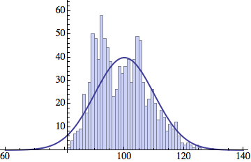

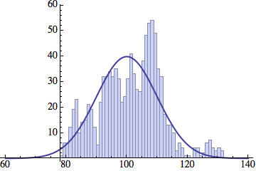
The curve is the Gaussian distribution with the mean equal to the number of cycles T and the standard deviation equal to the square root of T.
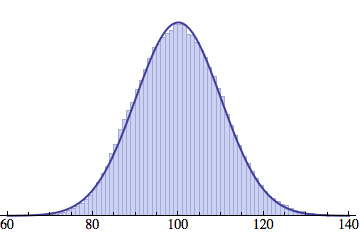
Averaging over 100 different runs (each with a population of 1000) gives a distribution that is nicely reproduced by the Gaussian curve:
And here is an animated GIF file showing the evolution of the generation distribution with time (in cycles of N deaths and births).
Joe Felsenstein pointed out if we follow the distribution of generations to times t longer than N, we will find that its width stops growing and remains around the square root of N/2. (Here is also my take on it.) The animated GIF below shows longer-term behavior of the distribution, to t=1000 in a population of N=1000. You can see clearly that toward the end of this interval the distribution is narrower and taller than the Gaussian it is supposed to follow.
Let me be more precise. The asymptotic expected within-population variance of generation number will be about 2(N-1) (and of course standard deviation the square-root of that). You will need to get past step 2N^2 a ways to see this (I’d go several times that), and of course the further beyond it you get, the more difference you will see between the overall variance and the within-population variance.
The system being stochastic, the actual variance will wander up and down around that value.
I have discovered a wonderful proof of this, but the margins of this blog are too small to contain it …
Joe Fermatstein?
I think that my value of 2N-2 for the asymptotic variance of the within-population variance was wrong. Instead half that: N-1.
Well, a bit off. (N-1)^2 / N. Which is (1 – 1/N) of the previous value. I am converging on the right answer.
I think I understand where that comes from. It has to do with the subject of the previous thread, fixation by neutral drift.
After generations, all of the M&Ms will be descendants of one and the same original M&M. (One can see that by starting with all original M&Ms having different colors; after about N generations, all M&Ms will be of the same color.)
In fact, at any point in time all of the M&Ms will be descendants of one M&M that lived about generations ago. (The proof goes along the same lines. Mark all M&Ms with different colors at time
  and see what happens at time
  .)
.)
So, even though the population has existed for generations, their ancestries were only independent for the last
  generations. Prior to that, they all had the same ancestors. So
  is the effective time during which their generation numbers were spreading out, not
  . For this reason the standard deviation of generations will only be
  , rather than
  .
.
Of course, the above assumes that exceeds
  . If it’s the other way around then we can’t go back
  generations, so the spread of generations will be
  . In my numerical experiments, I used
  = 1000 and
  from 0 to 100. So the width increased as
  . Had I waited longer, it would saturate at
  after about
  generations.
This is a marvelous toy model! Joe, many thanks for pointing out its hidden feature!
My numerics seem to converge on the asymptotic variance of N/2.
olegt,
Yep. Being mathematically somewhat inept, I visualise it, as a population of replicators hypothetically starting out as a single dot, an individual whose net output must have exceeded 1. Every individual in subsequent populations traces its ancestry back to it, through a varying number of copying steps. A succession of populations describes an approximate cone until the environment is saturated, at which point the stacking of successive populations forms an approximate cylinder, within which new cones are initiated which either come to occupy the full dimensions of the cylinder, or are snuffed out by other expanding cones (this is all without selection, of course).
A fresh bag of M&M’s is the cross-section through the cylinder whose prior state we have forgotten. If we arbitrarily decide that they all form the same generation, g0, we have reset the ‘generation clock’ and eliminated variance, and time must elapse before the spread of variances regains equilibrium, in the progression to which the spreads can be quite wide, as different lineages trace back to different g0 individuals, and small-number effects dominate. Once we have reached fixation of an ancestor, there is a limit to how many different paths to it can be represented within N members.
Two things. First of all by asking “who” nature is, is to ask a loaded question. There’s no good reason to think it is a “who”.
Second. We don’t even have to go into the whole naturalism/supernaturalism distinction. We need merely observe that a phenomenon takes place, a process of interactions between organisms, their genomes and their environment.
That is what we observe, yes. There’s no good reason to think this is somehow a miraculous happenstance in need to some kind of “had to have been designed otherwise it could not work”-explanation. Particularly because we frequently observe that this process doesn’t result in the “right” quantities of variation. Most life that has ever lived has gone extinct.
On the global scale, life is spread out enough and diverse enough for some kind of life to be able to persist, almost no matter what were to happen to our planet. This is all the explanation we need. There’s no need to add additional entities to this picture, it doesn’t explain it any more or any better, it only complicates things and it cannot be falsified. The rest is puddle-thinking.
Yes, I think I was off by 2. Oh the joys of doing theory empirically (or perhaps I should say, of offloading my argument-checking onto you).
Let’s try: (N-1)^2 / (2N)
Of course that is close to N/2, but it won’t be just N/2 since the within-population variance must be zero when N=1.
Joe Felsenstein,
A consequence of the variable being discrete? Individuals aren’t infinitely subdivisible.
It also makes sense for N=2. At any time the population consists of a parent and its child. Their generations are consecutive, and
and  , so they differ from the mean
  by 1/2 each. This gives a variance of
in agreement with your conjecture.
Good check of my formula.
By the way, watching the animated GIF in this post, I think I can see, as the distribution gets towards the right side of the plot, that the within-population genetic variance is smaller than the prediction of a variance of t.
I can’t seem to be able to embed an image in a comment, so here is a link to a plot of variance versus time (in generations) on a log-log scale. A population of N = 100 observed until t = 1000. The variance is noisy for individual runs, so I averaged it over 1600 runs.
After an initial linear rise, the variance saturates at N/2 = 50.
In case anyone wants to write code to simulate it, it should be relatively straightforward to predict the amount of variability maintained by mutation in the face of genetic drift in this Moran model.
But we’d have to agree on a tractable model of mutation. I suggest that each newborn (the one in each generation that is an offspring) have a probability u of changing to one of the other K-1 possible colors. If that can be simulated, I’ll work out the formula. It would be based on a 1969 result by Motoo Kimura.
Looks good, but can you rule out that it actually saturates at 49.005, which is (99^2)/200 ?
Staring at the GIF, I think I can see the pattern underlying my previous observation (that runs that get to fixation more quickly for a given N have higher spreads (as clumsily represented by maxima and minima) than those that took longer).
The left hand side of the GIF shows significant outliers outside the curve; towards the right these are lost, as the population settles (back) into an equilibrium, having been distorted by assigning Gen0 with no variance (in anything).
It probably does saturate at , rather than
  , but the data is still too noisy to tell the difference.
Here is a histogram for a population of N=1000 after t=1000 generations (the GIF in the OP only goes to t=400). You can see clearly that the histogram is narrower and taller than a Gaussian curve with a variance of t.
ETA. Added a longer-term animation to the OP.
Joe Felsenstein,
Why that particularly? One could have a set of possible numbered ‘colours’ starting at N+1 and incremented for each mutant (such that every mutant is unique, and 1 thru N have been reserved for the current population, even if not all used). This is probably closer to the reality, where mutations tend overwhelmingly to fall outside those represented in the current population. But it may be less tractable mathematically?
That an even-more-tractable model and would be fine. It is called the “infinite-alleles model” and is widely used in theoretical work on neutral mutations.
It is just that I suspected that it would be hard for anyone to draw that many colors.
Joe Felsenstein,
It’s hard for me to draw any! That’s why I go for a painting-by-numbers version. Allele is a numeric label in my models.
[I can’t edit posts I make at work but can from home. The Click to Edit and Request Deletion buttons don’t show. Takes me an hour to get home; never quick enough!].