Counting generations of M&Ms

Posted on January 14, 2014 by olegt

Allan Miller’s post Randomness and evolution deals with neutral drift in the Moran model applied to a bag of M&Ms. Much of the discussion has focused on the question of counting generations in a situation where they overlap. I think it’s a good idea to divert that part of the discussion into its own thread.

Here are the rules. Start with a population of N M&Ms. A randomly chosen M&M dies. Another randomly chosen M&M gives birth to a child M&M. Repeat.

Because the focus of this thread is generation count and not fixation, we will pay no attention to the colors of M&Ms.

How do we count generations of M&Ms?

My recipe. Count the number of deaths and divide by N. It can be motivated as follows. A single step (one death and one birth) replaces 1 out of N M&Ms. We need at least N steps to replace the original M&Ms.
Joe Felsenstein’s recipe. The original M&Ms are generation 0. Children of these M&Ms are generation 1. Children of generation n are generation n+1. The generation count at any given point is obtained by averaging the generation numbers of the population.
Replacement recipe. A generation passes when an agreed-upon fraction of the current population (e.g., 90 percent) is replaced.

Numerical experimentation with the Moran model shows that recipes 1 and 2 give similar generation counts in a large population, say, N=1000. I suspect that the third recipe will give a generation count that differs by a numerical factor. In that case one can select the “right” fraction that will yield the same count as the first two recipes.

Have at it.

ETA. Let us define generations as Joe did (definition 2 above): the original organisms are generation 0, their children are generation 1, and so on. Let us call N deaths and N births one cycle.

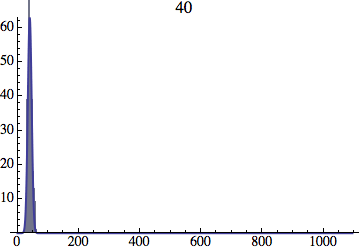
I wrote a simple Mathematica script that plots the distribution of generations after a given number of cycles. Here are a few representative histograms for N=1000 organisms after T=100 cycles.

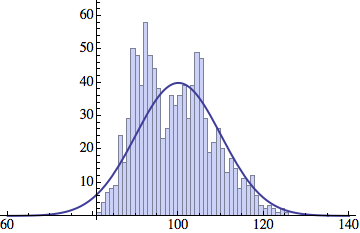
The curve is the Gaussian distribution with the mean equal to the number of cycles T and the standard deviation equal to the square root of T.

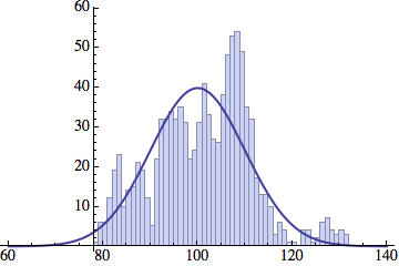
Averaging over 100 different runs (each with a population of 1000) gives a distribution that is nicely reproduced by the Gaussian curve:

And here is an animated GIF file showing the evolution of the generation distribution with time (in cycles of N deaths and births).

Moran-animation-1

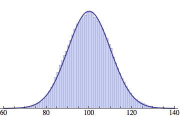
Joe Felsenstein pointed out if we follow the distribution of generations to times t longer than N, we will find that its width stops growing and remains around the square root of N/2. (Here is also my take on it.) The animated GIF below shows longer-term behavior of the distribution, to t=1000 in a population of N=1000. You can see clearly that toward the end of this interval the distribution is narrower and taller than the Gaussian it is supposed to follow.

Moran-animation-4

171 thoughts on “Counting generations of M&Ms”

Allan Miller on January 17, 2014 at 12:18 pm said:

Blas,

As we have found specific mechanism for adaptation changes it is still possible that microevolution is a built-in mechanism of the life forms.

Microevolution, as minimally represented by this ‘baseline’ model of neutral drift, upon which allele selective differentials superimpose, is an unavoidable consequence of populations being finite. It does not need to be ‘built in’ to anything. It’s memoryless, and (given an input of novel variation and no extinction) perpetual.
Neil Rickert on January 17, 2014 at 12:35 pm said:

Allan Miller: One area where I find population genetics to have been misleading is in the matter of the “twofold cost of sex”.

I never looked closely into that argument. To me, it seems to be something like a claim that it costs more to operate my car, if I put gas in the tank.
Blas on January 17, 2014 at 12:43 pm said:

Alan Fox: There are quite a few known factors too, though it is only germinal mutations that can be inherited.

Well I were thinking in specific increase of variability in gene areas induced by strees or epigenetic mechanisms.
Blas on January 17, 2014 at 12:45 pm said:

Allan Miller:
Blas,

Microevolution, as minimally represented by this ‘baseline’ model of neutral drift, upon which allele selective differentials superimpose, is an unavoidable consequence of populations being finite. It does not need to be ‘built in’ to anything. It’s memoryless, and (given an input of novel variation and no extinction) perpetual.

Yes, but it is a very ineficient process as in an isolated population of 100 reproductive members only 1 every 100 neutral mutations get fixed.
olegt on January 17, 2014 at 1:02 pm said:

Blas: Yes, but it is a very ineficient process as in an isolated population of 100 reproductive members only 1 every 100 neutral mutations get fixed.

And in an isolated population of 1000, only 1 out of every 1000 neutral mutations gets fixed. And if we get a population of 10,000… Sounds like neutral mutations will have less chance to get fixed in larger populations?

That, however, is only one side of the story, Blas. Here is the other side.

As the population size grows, so does the number of mutations. If the probability of a neutral mutation to appear in one organism is 1/50 then in a population of 100 we will have 2 mutations per generation. Each gets fixed with the probability 1/100, so the chance to see a new fixed mutation is 0.02 per generation.

With a population of 1000, we expect 20 mutations per generation. Each gets fixed with the probability 1/1000, so once again we expect 0.02 fixed neutral mutations per generation.

More generally, if the probability of a mutation is p in one organism then we have pN mutations per generation. Each gets fixed with a probability of 1/N, so we have p neutral mutations fixed per generation.
OMagain on January 17, 2014 at 1:09 pm said:

Blas: microevolution is a built-in mechanism

Built in by who?
Alan Fox on January 17, 2014 at 1:09 pm said:

Blas: Well I were thinking in specific increase of variability in gene areas induced by strees or epigenetic mechanisms.

Apparently stress mutation is well studied and documented. What happens is that mutations become more frequent. There is no directed response to stress.

ETA

Just to clarify, there is no input from the changed environment that brings about mutations that would be designed to be “fitter” in the new circumstances. The idea is that more mutations means more possibilities that selection will find a “fitter” solution.
Allan Miller on January 17, 2014 at 1:20 pm said:

Alan Fox,

It’s the have-cake eat-cake school of thought. Mutations are all bad and lead to nothing except when they are a built-in response to a stress, in which case they’re grrrrrrreat!

The possibility exists of a genome-resident mutation control mechanism, but one would need to distinguish it from a simple loss of fidelity under stress.
Allan Miller on January 17, 2014 at 1:23 pm said:

Neil Rickert,

http://en.wikipedia.org/wiki/Evolution_of_sexual_reproduction#Two-fold_cost_of_sex

No, it’s basically the fact that asexuals can outproduce gendered sexuals, all else being equal, two for one.
Blas on January 17, 2014 at 1:39 pm said:

olegt: And in an isolated population of 1000, only 1 out of every 1000 neutral mutations gets fixed. And if we get a population of 10,000… Sounds like neutral mutations will have less chance to get fixed in larger populations?

That, however, is only one side of the story, Blas. Here is the other side.

As the population size grows, so does the number of mutations. If the probability of a neutral mutation to appear in one organism is 1/50 then in a population of 100 we will have 2 mutations per generation. Each gets fixed with the probability 1/100, so the chance to see a new fixed mutation is 0.02 per generation.

With a population of 1000, we expect 20 mutations per generation. Each gets fixed with the probability 1/1000, so once again we expect 0.02 fixed neutral mutations per generation.

More generally, if the probability of a mutation is p in one organism then we have pN mutations per generation. Each gets fixed with a probability of 1/N, so we have p neutral mutations fixed per generation.

As I said. You have one neutral mutation fixed every 50 generations. And 99 neutral mutations get lost. A very ineficient process for variability.
Neil Rickert on January 17, 2014 at 1:40 pm said:

Allan Miller: No, it’s basically the fact that asexuals can outproduce gendered sexuals, all else being equal, two for one.

Yes, I know that’s the reasoning given. But it is based on selfish gene thinking. It assumes that the purpose of reproduction is replicate one’s genes. I’m more inclined to think of reproduction as part of sustaining the population.
Blas on January 17, 2014 at 1:40 pm said:

OMagain: Built in by who?

Who cares? Crossing over during meiosis isn´t a built-in mechanism for variation?
Blas on January 17, 2014 at 1:42 pm said:

Alan Fox: Apparently stress mutation is well studied and documented. What happens is that mutations become more frequent. There is no directed response to stress.

ETA

Just to clarify, there is no input from the changed environment that brings about mutations that would be designed to be “fitter” in the new circumstances. The idea is that more mutations means more possibilities that selection will find a “fitter” solution.

There are papers that shows that, in some cases, the increase of mutation is in specific areas of specific genes.
olegt on January 17, 2014 at 1:43 pm said:

Blas: As I said. You have one neutral mutation fixed every 50 generations. And 99 neutral mutations get lost. A very ineficient process for variability.

Neutral drift isn’t a source of variations. Mutations are.
Alan Fox on January 17, 2014 at 1:51 pm said:

Blas: There are papers that shows that, in some cases, the increase of mutation is in specific areas of specific genes.

I’ve no reason to think otherwise. What I am saying that the only ways that mutations (non-lethal) get into the population is by selection or drift. Many mutations arise but few are chosen. 😉

ETA to include drift.
Allan Miller on January 17, 2014 at 2:04 pm said:

Neil Rickert,

Yes, I know that’s the reasoning given. But it is based on selfish gene thinking. It assumes that the purpose of reproduction is replicate one’s genes. ’m more inclined to think of reproduction as part of sustaining the population.

Reproduction is the sine qua non of Life, Evolution and Everyfink! The fact that ‘a population’ results is a consequence of average outputs in excess of 1. It has the effect of sustaining a population, but that cannot be its primary ‘purpose’.

The 2-fold cost is not explicitly based on Selfish-genism, though it can be: each gene has only half a chance of being in the next gamete. But the cost of males is more subtle – each gene spends half its life in each gender, so males are not intrinsically costly to genes. That cost is a cost of whole-organism production and replacement.

The whole-organism view and the gene’s-eye view both miss the fact that there is a little organism right in between them at the heart of the process: the haploid. We are part of its life cycle, not the other way round.
Allan Miller on January 17, 2014 at 2:08 pm said:

Blas,

Who cares?

Who cares? Who bleeding cares? Sheesh. No-one, obviously. Just A Passing Designer, identity and present and future interest of no importance!

Crossing over during meiosis isn´t a built-in mechanism for variation?

No
OMagain on January 17, 2014 at 2:09 pm said:

Blas: Who cares?

Not you, evidently.
Allan Miller on January 17, 2014 at 2:12 pm said:

Blas,

As I said. You have one neutral mutation fixed every 50 generations. And 99 neutral mutations get lost. A very ineficient process for variability.

By what criterion?
Blas on January 17, 2014 at 2:33 pm said:

olegt: Neutral drift isn’t a source of variations. Mutations are.

If you want a very inefficient process to fix variations.
Blas on January 17, 2014 at 2:35 pm said:

Allan Miller:
Blas,

By what criterion?

If you produce 100 and you get one which criterion will not call that inneficient. Off course you always will get mor inneficient process but that do not make this efficient. May be less inneficient
Allan Miller on January 17, 2014 at 2:53 pm said:

Blas,

To put it another way: Who cares? If the process is adjudicated inefficient by Poster X Of The Internet, what kind of a problem is that for Nature?

Nature is actually working hard to eliminate variation, actively and passively, which is why it has all manner of proofreading and other mechanisms to keep mutation rate as low as it is, and why population resampling has the effect it does. It would depend what entity you talked to as to whether the variations that actually get into the population do so ‘inefficiently’ or not.
OMagain on January 17, 2014 at 3:15 pm said:

Blas: If you want a very inefficient process to fix variations.

Luckily there’s lots of time available.
petrushka on January 17, 2014 at 3:21 pm said:

I would point out that neutral mutations are called neutral because they have no discernible effect on reproductive success. That means they passed through the sieve of purifying selection.

They are still selected, just not differentially selected.
Joe Felsenstein on January 17, 2014 at 3:32 pm said:

Allan Miller:
Joe Felsenstein,

One area where I find population genetics to have been misleading is in the matter of the “twofold cost of sex”. I think it’s an illusion, though I have found myself in phoodoo’s position, the scorned outsider, when trying to defend that. It’s a complicated argument, but I think even such eminent people as Williams, Maynard Smith and Hamilton missed important considerations in their formulation, which still has some scratching their heads over what might be the offsetting “twofold benefit” today. There isn’t one, IMO.

Potentially unmasking myself as a crank, and a matter for another thread, perhaps!

This is off-topic here of course, but it is an area in which I have worked (my work was mostly on natural selection for recombination). I do think I know the logic of the argument for the two-fold cost of “sex”. I do teach classes explaining it.

If you could email me (my email address is easily available on the web) I’d be happy to hear your argument and give you some reactions.
keiths on January 17, 2014 at 4:01 pm said:

Joe, to Allan:

If you could email me (my email address is easily available on the web) I’d be happy to hear your argument and give you some reactions.

Could you guys do it as a new thread, instead of a private email exchange? That way the rest of us could benefit from the discussion.

If you’re concerned that the thread might get phoodoo’ed, you could always conduct the email exchange privately but then post it as a new thread.
Allan Miller on January 17, 2014 at 4:46 pm said:

Joe Felsenstein,

I do think I know the logic of the argument for the two-fold cost of “sex”. I do teach classes explaining it.

Yes, I’m aware of your involvement in the field, and the somewhat hubristic nature of my claim in light of the fact that everyone and their dog has chewed this issue to the bone. I appreciate your offer to examine my argument, and will put some thought into that.
Joe Felsenstein on January 17, 2014 at 4:50 pm said:

Allan Miller:
Joe Felsenstein,

…

appreciate your offer to examine my argument, and will put some thought into that.

I am willing to participate either in discussion of a post here, or in an email exchange. Your decision.
Allan Miller on January 17, 2014 at 5:16 pm said:

Joe Felsenstein,

OK, thanks. As I have a tendency to over-edit myself, it won’t be too soon!

I’m happy to let TSZ-ers see it (if I’m embarrassingly wrong, it would hardly be the first time!), but will probably go via email in the first instance.
Allan Miller on January 17, 2014 at 6:22 pm said:

For anyone who remains interested, I posted a single figure on the other thread regarding the discrepancy between methods 1 (estimate, by deaths/N) and 2 (actually keep count and then analyse the final population). Here are some more.

The 2 will differ on any run, because when you kill an individual, you affect the counted mean by a different amount depending on its generation count, to which deaths/N is blind.

200 runs at N=10,000 gives

Method 1 mean 10163 generations S/D 5612
Method 2 mean 10131 generations S/D 5608.
The greatest range in counted minimum/maximum for the 200 runs was 7% of the mean; the lowest 0.5%.

Method 1 overestimated in 66.5% of runs. Whether that’s significant, I don’t know.
Blas on January 17, 2014 at 6:43 pm said:

Allan Miller:
Blas,

To put it another way: Who cares? If the process is adjudicated inefficient by Poster X Of The Internet, what kind of a problem is that for Nature?

Nature is actually working hard to eliminate variation, actively and passively, which is why it has all manner of proofreading and other mechanisms to keep mutation rate as low as it is, and why population resampling has the effect it does. It would depend what entity you talked to as to whether the variations that actually get into the population do so ‘inefficiently’ or not.

So Nature, I do not know who it is, works in order to reduce the variation but also produce variation. And is good that this Nature reduce the variation and is also good that produce variation. Off course Nature is able to produce the right quantities of variation.
Patrick on January 17, 2014 at 6:49 pm said:

Allan Miller:
For anyone who remains interested, I posted a single figure on the other thread regarding the discrepancy between methods 1 (estimate, by deaths/N) and 2 (actually keep count and then analyse the final population).Here are some more.

The 2 will differ on any run, because when you kill an individual, you affect the counted mean by a different amount depending on its generation count, to which deaths/N is blind.

200 runs at N=10,000 gives

Method 1 mean 10163 generations S/D 5612
Method 2 mean 10131 generations S/D 5608.
The greatest range in counted minimum/maximum for the 200 runs was 7% of the mean; the lowest 0.5%.

Method 1 overestimated in 66.5% of runs. Whether that’s significant, I don’t know.

Allan,

Did you have a setting for maximum number of deaths or did you let the runs go to fixation? Did you use an even distribution of initial colors plus one black?

Thanks.
Patrick on January 17, 2014 at 6:51 pm said:

So Nature, I do not know who it is,…

Why would you assume it is a who?

Off course Nature is able to produce the right quantities of variation.

Nope. Sometimes species go extinct when they can’t adapt.
Allan Miller on January 17, 2014 at 8:00 pm said:

Patrick,

I just let simple probability take care of death, as in the basic Moran model. This carries the slightly artificial flavour that the oldest individual in a run increases with increasing N, but I don’t think this has a huge effect on the outcome.

Basically, the probability of one of N individuals surviving N random deaths is 1/e [((N-1)/N)^N] -> 36.78% at increasing N. Thus 63.32% of the population dies in its first ‘year’ (if we arbitrarily assign a year as the time taken to replace N individuals).

86.4% die in their first 2 years.
95% die in their first 3 years
98% die in their first 4 years

and so on. This means that the population of survivors is strongly weighted towards youngsters. The series above obviously stops eventually for finite N – zero individuals exceed a certain threshold. But that threshold goes up as N does. Survival for 8 years is possible for an average 3.5 individuals in a population of 10,000, but if you want more than 1 every 3 runs for 1,000, you’d have to make offerings to the Probability Gods.

A similar relation holds for offspring number, though the probabilities are combined – p(survival) and p(birth). The resultant is a halving per N, so again the rare extremes don’t argue for a cap.

As for the single colour question, I ignore colour completely; it can be a bit of a .. umm … red herring. The start of my runs has N different individuals, individually labelled, so they are all essentially a different colour, evenly distributed. The run stops when one of them has fixed. I’m interested in the whole ‘cone’ of fixation. Starting at a particular frequency other than 1/N is effectively starting at the cross-section through a set of such cones that started prior to the run.

But for mutation, one could usefully turn the process inside out – initially label every member identically, and have a mutation rate parameter, then halt when the initial label has disappeared through appearance and fixation of one or more mutants. Such a version of OMagain’s sim, starting all white, would be an effective demo of the ability of the process to fix novelty by exactly the same method by which such variation is eliminated (hint, hint!).
Allan Miller on January 17, 2014 at 8:05 pm said:

Blas,

So Nature, I do not know who it is, works in order to reduce the variation but also produce variation. And is good that this Nature reduce the variation and is also good that produce variation. Off course Nature is able to produce the right quantities of variation.

It just happens. It’s neither good nor bad, nor always enough, too much or too little. It simply has consequences.
OMagain on January 17, 2014 at 8:18 pm said:

Allan Miller: Such a version

I’ll do that. I should be putting up a new version this weekend, I’ll add this in as a variant. More soon!
Zachriel on January 18, 2014 at 7:25 pm said:

Allan Miller: Basically, the probability of one of N individuals surviving N random deaths is 1/e [((N-1)/N)^N] -> 36.78% at increasing N.

Question. The original simulation had replacement level reproduction. How did you handle the extra deaths to maintain population?
Allan Miller on January 18, 2014 at 7:54 pm said:

Zachriel,

The original simulation had replacement level reproduction. How did you handle the extra deaths to maintain population?

Mine has that too. Birth and death are alternate processes; occurring singly, so N never varies, except momentarily. An individual is randomly selected to reproduce, and one to die. The slot vacated by the fatality (which could be the parent) is filled by the newborn.

After N such random events, 36.78% of an original N slots would still contain their original occupant, and hence have survived for 1 ‘age unit’, the time taken for N replacements. 36.78% of those would survive another, and so on.
Zachriel on January 18, 2014 at 9:21 pm said:

Allan Miller: The slot vacated by the fatality (which could be the parent) is filled by the newborn.

Whether the fatality is by senescence or by replacement. Thanks!
olegt on January 18, 2014 at 9:36 pm said:

I have added several representative histograms of the age distribution to the opening post. In these examples, N = 1000 organisms went through T = 100 cycles. Here one cycle = N deaths and N births. The typical age is approximately T and the width of the age distribution is roughly the square root of T.

If my TeX skills do not fail me, I will show below that this is what statistical analysis predicts for the Moran model.
olegt on January 18, 2014 at 10:40 pm said:

Added to the opening post an animated GIF file showing the evolution of the age distribution with time measured in cycles (N deaths and N births).
olegt on January 19, 2014 at 12:47 am said:

Let’s sort out the mathematics of the model.

Although the exact number of M&Ms in generation $x$ at any point is impossible to predict, it is possible to predict the average number of such M&Ms that we can expect. Let us denote the expected number of M&Ms of the original generation $n_0$ . The expectation number of M&M of the first generation (their children) is $n_1$ , and so on. At time $t=0$ , all M&Ms are in this generation, i.e., $n_0 = N$ and $n_1 = n_2 = \ldots = 0$ .

The number of the original M&Ms $n_0$ can only go down: they can only die. If we observe the bag for a short period of time $dt$ , the number of deaths of the original M&Ms will be proportional to the amount of time (the longer we watch, the more deaths) and to the number of these M&Ms. These proportionalities are expressed mathematically as $d n_0 = - C n_0 dt$ . (The minus sign says that the number of the M&Ms is going down.)

We still have to determine the numerical constant $C$ . This can be done by considering the situation at time $t=0$ , when $n_0 = N$ . If we choose the unit of time to be one cycle, or $N$ deaths, then there will be 1 death during time $dt = 1/N$ . So $dn_0 = -1$ for $n_0 = N$ and $dt = 1/N$ . This tells us that $C=1$ is the right choice. Hence

$d n_0/dt = - n_0.$

This differential equation has a simple solution: $n_0(t) = \mathrm{const} \times e^{-t}$ . The constant is determined from the initial condition, $n_0(0) = N$ . We thus obtain

$n_0(t) = N e^{-t}.$

We now see that the expected number of the original M&Ms (generation 0) decays exponentially in time. After t=1 cycle ( $N$ deaths), we are left with $N/e = 0.37 N$ M&Ms. After $t=3$ cycles, $n_0 = N e^{-3} = 0.05 N$ M&Ms.
(continued)
olegt on January 19, 2014 at 1:22 am said:

Next we compute how the expected number of M&Ms in the first generation. Their number changes for two reasons: it increases when an original M&M (genereation 0) gives birth and decreases when a member of generation 1 dies. The increment of $n_1$ during a short period of time $dt$ is thus $d n_1 = + n_0 dt - n_1 dt$ . This yields a differential equation

$d n_1/ dt = n_0 - n_1.$

We have already determined that $n_0 = N e^{-t}$ , so

$d n_1/ dt = N e^{-t} - n_1.$

This differential equation can also be solved. For the initial condition $n_1(0) = 0$ , we obtain

$n_1(t) = N e^{-t} t.$

The number of M&Ms in generation 1 first grows linearly with time, as long as the parent generation is alive and reproducing. Eventually the parents die out and cut off the supply of new M&Ms. At that point, generation 1 will start declining and eventually die out, too.
olegt on January 19, 2014 at 1:39 am said:

We can continue doing this for further generations of M&Ms.

The number of M&Ms in generation $x$ increases when one of their parents gives births and decreases when one a member of generation $x$ dies. Mathematically,

$d n_x / dt = n_{x-1} - n_x.$

By the time we consider generation $x$ , we have already solved for $n_{x-1}(t)$ , which we plug into the above equation and solve for $n_x(t)$ , which initially is zero, $n_x(0) = 0$ . In this way we find that

$n_x(t) = N e^{-t} t^x/x!$

At any given time $t$ , the numbers $n_x$ form a Poisson distribution. From the known properties of that distribution we can determine the mean generation of M&Ms as being simply $t$ . At time $t=1$ , the average generation is 1, at $t=2$ , it is 2, and so on. This confirms what we have suspected all along: counting generations as $N$ deaths (definition 1) and counting them as Joe Felsenstein did (definition 2) should give the same result, at least on average.

We can also determine the width of the generation distribution as the square root of the variance. This yields the width equal to $\sqrt{t}$ . So, after 100 cycles we expect to find M&Ms of generations 90 to 110.
Patrick on January 19, 2014 at 9:02 pm said:

olegt:

We can also determine the width of the generation distribution as the square root of the variance. This yields the width equal to $\sqrt{t}$ . So, after 100 cycles we expect to find M&Ms of generations 90 to 110.

I just tried this with my implementation of the model. With a population size of one thousand, running until there are one hundred thousand deaths, over two thousand trials, I find the minimum generation number to be 55, the maximum to be 147, with a mean very close to 100 with a standard deviation of about 3.

The mean minimum generation is around 75 and the mean maximum is around 125.

Using the difference between the minimum and maximum of each run as the range, I get a minimum range of 31 and a maximum of 72, with a mean of about 48 (and a big standard deviation of over 6). If I understand your math, this should actually be the square root of the number of generations which equals 10, correct?

Is my implementation or understanding wrong?
Joe Felsenstein on January 19, 2014 at 9:18 pm said:

olegt,

Bravo! Excellent job. Of course, I can come up with a more exact solution, and show that it is obvious (after the fact. There is a Felsenstein’s Law that states that all true results are obvious — after the fact. The harder task is to have them be obvious before the fact.)

Consider a Moran model with N M&M’s, and each step consists of drawing one, duplicating it (and labeling the new one as being one generation later than its parent), and then removing one of the M&M’s other than these two and having the new one replace it. Suppose that we have a population just after time step S. Now take a random M&M and consider it or its ancestors in all previous generations. Going back along this chain to the starting population, which is at time step 0, we can see that in each of populations S, S-1, S-2, …, 1 there is a probability 1/N that the M&M is a newborn. And these events are independent.

So we can then say that the generation number of a randomly chosen M&M from time step S is drawn from a binomial distribution (the distribution we use to model independent coin tosses) with S coin tosses each with Heads probability 1/N. The number of Heads is the generation number of the randomly chosen M&M that we draw in time step S. The variance of that generation number will then be S(1/N)(1-1/N) or (S/N)(1-1/N).

If we consider a series of populations with larger and larger N, for each considering “time” as t = S/N, it is well known that the binomial distribution converges to a Poisson distribution with expectation t, giving olegt’s result.

I had gotten as far as seeing that the distribution of generation numbers would have a variance that increased linearly, but only after I saw olegt’s analysis did this going-back argument occur to me.

I will add one more prediction, though the argument that leads to it is will not fit here. The ever-increasing variance of the distribution of generation numbers is true for a collection of populations, when we compute the variance by combining all their M&M’s. But within any one population, the within-population variance will approach an asymptote and come to vary around it. The height of that asymptote will be proportional to N. (All of that comes from considering a coalescent, which leads us to the fact that the generation numbers in two M&M’s in the same population are strongly correlated).
Allan Miller on January 19, 2014 at 9:40 pm said:

Patrick,

I think your runs may be too short to converge on the expected result. You’re only doing N/10 generations. Analysing my distributions, from 200 replicates of N=10000, and ordering by spread as a percentage of the mean, the broadest spreads occurred on the shortest runs (I stop at fixation).

I just tried re-analysing based on the actual max/min vs mean plus-or-minus its square root, and runs to the left of the graphs (tending to be the longer) all stay comfortably within the expected variance; those to the right (the shorter) tend to be more likely to fall outside.
olegt on January 19, 2014 at 10:18 pm said:

Patrick: Using the difference between the minimum and maximum of each run as the range, I get a minimum range of 31 and a maximum of 72, with a mean of about 48 (and a big standard deviation of over 6). If I understand your math, this should actually be the square root of the number of generations which equals 10, correct?

Is my implementation or understanding wrong?

Hi Patrick,

The smallest and largest numbers in a distribution can be pretty far apart. In your case, they are typically $3\sigma$ away from the mean in each run. Getting a deviation of $3\sigma$ or more in a Gaussian ensemble has a chance of 1 in ~~300~~ 400, so it’s quite likely to happen in a population of 1000. So that’s quite all right.

Figures added to the opening post show that each population has a distribution that doesn’t really agree with the theoretical curve. However, if you average over many runs, the curve fits beautifully. I have just added one more figure to the OP showing that.

ETA. In my 100 repeats of the experiment (each with 1000 M&Ms to time t=100), the minimum number of generations was 64 and the maximum 136, both deviating by 36 from the mean of 100. And in the next installment of 100 repeats I found a member of the 146th generation. That’s a deviation of $4.6\sigma$ from the mean, which is expected to happen about once in 237,000 cases, and I had 100,000. So that’s pretty much in the ballpark.
olegt on January 19, 2014 at 10:35 pm said:

Joe Felsenstein: So we can then say that the generation number of a randomly chosen M&M from time step S is drawn from a binomial distribution (the distribution we use to model independent coin tosses) with S coin tosses each with Heads probability 1/N. The number of Heads is the generation number of the randomly chosen M&M that we draw in time step S. The variance of that generation number will then be S(1/N)(1-1/N) or (S/N)(1-1/N).

Ooooh, that’s a very nice argument, Joe!

Of course, being a theoretical physicist, I abhor discrete mathematics. So, rather than first getting a binary distribution and then going to a Poisson one (in the large- $N$ limit), I went straight to the continuum limit.

In fact, my first derivation was even farther away from yours: I derived a Gaussian distribution by treating the generation number as a continuous variable. Starting with the equation

$d n_x/dt = n_{x-1} - n_x,$

I make the generation number $x$ a continuous variable, so $n = n(x,t)$ :

$\partial n(x,t)/\partial t = n(x-1,t) - n(x,t).$

Then I Taylor-expand $n(x-1) \approx n(x) - d n(x)/d x + \frac{1}{2} d^2 n(x)/d x^2$ and obtain the convection-diffusion equation:

$\frac{\partial n}{\partial t} = - \frac{\partial n}{\partial x} + \frac{1}{2} \frac{\partial^2 n}{\partial x^2}.$

Its solution is a Gaussian packet centered at $x=t$ with the width $\sqrt{t}$ (i.e., both the mean and variance are equal to $t$ ):

$n(x,t) = \frac{N}{\sqrt{2\pi t}} \exp{\left(- \frac{(x-t)^2}{2t} \right)}.$

That’s the theoretical curve used in the figures appended to the opening post.

Of course, the Gaussian distribution obtains from the Poisson one for large $t$ .
Patrick on January 19, 2014 at 10:44 pm said:

Allan Miller:
I think your runs may be too short to converge on the expected result. You’re only doing N/10 generations.

Thanks, I think. Between this comment and Joe Felsenstein’s most recent prediction, I’m going to have my CPUs running hot all night.