David Nemati and Eric Holloway, “Expected Algorithmic Specified Complexity.” Bio-Complexity 2019 (2):1-10. doi:10.5048/BIO-C.2019.2. Editor: William Basener. Editor-in-Chief: Robert J. Marks II.

Eric Holloway has littered cyberspace with claims, arrived at by faulty reasoning, that the “laws of information conservation (nongrowth)” in data processing hold for algorithmic specified complexity as for algorithmic mutual information. It is essential to understand that there are infinitely many measures of algorithmic specified complexity. Nemati and Holloway would have us believe that each of them is a quantification of the meaningful information in binary strings, i.e., finite sequences of 0s and 1s. If Holloway’s claims were correct, then there would be a limit on the increase in algorithmic specified complexity resulting from execution of a computer program (itself a string). Whichever one of the measures were applied, the difference in algorithmic specified complexity of the string output by the process and the string input to the process would be at most the program length plus a constant. It would follow, more generally, that an approximate upper bound on the difference in algorithmic specified complexity of strings $y$ and $x$ is the length of the shortest program that outputs $y$ on input of $x.$ Of course, the measure must be the same for both strings. Otherwise it would be absurd to speak of (non-)conservation of a quantity of algorithmic specified complexity.

For conventional computers, the shortest of programs immediately halts the computational process. The output is the empty string, no matter what string is input. However, the length of the program is not an approximate upper bound on the difference in algorithmic specified complexity of empty and nonempty strings. In “Evo-Info 4: Non-Conservation of Algorithmic Specified Complexity,” I showed that the empty string is, by some measures, infinitely greater in algorithmic specified complexity than all nonempty strings. My result not only refutes Holloway’s claims, but also destroys the prospect of establishing an alternative “conservation law” that holds for each and every measure of algorithmic specified complexity (ASC). Yet Nemati and Holloway frame Section 4 of their article as a response to my argument, saying that it “does not disprove conservation of ASC.” They neither state the result that I derived, nor venture even to cite the post containing it. Instead, they derive a new expression of “conservation of complexity,” obfuscating an application of different measures of algorithmic specified complexity to two strings. If they had made a direct comparison of their result to mine, then they necessarily would have exposed their change from one ASC measure to another. In a remarkable touch, at the end of the passage on display below, the authors attribute error to me in not pulling the switcheroo that they do.

The gist of the passage above is that the algorithmic specified complexity of a string “properly” depends on how the string is expressed. In my argument, the ASC measure is restricted in such a way that the algorithmic specified complexity of a string is infinite only when the string is empty. If we refer to the empty string as $\lambda$ (the lowercase Greek letter lambda), then Nemati and Holloway agree that the empty string is infinitely greater in algorithmic specified complexity than all nonempty strings. But if we instead refer to the empty string as $f(x),$ where $f$ is a function with $f(x) = \lambda$ for all strings $x,$ then the authors change the ASC measure in such a way that the algorithmic specified complexity of the empty string is negative. Their “conservation of complexity” inequality (43), in the passage above, is tacitly an upper bound on the difference in the ASC of $f(x),$ according to the modified measure, and the ASC of $x,$ according to the original measure. If you find it hard to believe that the authors would believe that the measure should depend on how a string is expressed, then you should read “Stark Incompetence,” the first part of my review of the article.

The next section of this post gives a simple explanation of algorithmic specified complexity, and then describes how the authors use the expression of a string to modify the ASC measure. The following two sections step through my annotations of the passage above, and delve into the misconception that the measure of algorithmic specified complexity should depend on the way in which a string is expressed. (There is some redundancy, owing to the fact that the sections originated in separate attempts at writing this post.) The final section, “Supplement for the Mathematically Adept,” not only provides details undergirding my remarks in the earlier sections, but also

tightens the “conservation of complexity” bound (43),
improves upon “the paper’s main result” (16), and
corrects some errors in Section 4.2.

The authors should cite this post, and note that it improves upon some of their results, in the statement of errata that they submit to Bio-Complexity. They have no excuse, when publishing in a scholarly journal, for omitting citations of posts of mine that they draw upon.

A provisional response

Was mich nicht umbringt, macht mich stärker.

— Friedrich Nietzsche, Maxims and Arrows, 8 [translate]

The significance of provisional is that I am suppressing some details. In later sections, you will get graduated doses of the straight dope, and hopefully will acquire greater and greater tolerance of it. However, there is one technical point that I cannot bring myself to suppress. The computer I refer to is “ordinary” in the sense that the shortest of all programs halts with the empty string as output, no matter what string is input. It is possible to contrive a computer for which the shortest program that merely halts is much longer than some other programs that halt. But what matters here is that there do exist computers for which the “do nothing but to halt” program is no longer than any “do something and halt” program.

As I have emphasized, algorithmic specified complexity is an infinite class of measures. The particular measure is determined by parameters referred to as the chance hypothesis and the context. The chance hypothesis corresponds to one scheme for recoding of data (strings of bits), and the context corresponds to another. It might be that the recoding of data $x = \mathtt{1101}$ in the scheme associated with the chance hypothesis is $\mathtt{101101},$ and that the recoding in the scheme associated with the context is $\mathtt{010}.$ The algorithmic specified complexity of the data is the difference in the numbers of bits in the two recodings of the data. In this case, the difference is $6 - 3 = 3$ bits. When Nemati and Holloway switch from one measure of algorithmic specified complexity to another, it is actually just the chance hypothesis that they change. So we will be concerned primarily with the chance hypothesis.

The chance hypothesis, so called, is an assignment $p$ of probabilities to data that might be encountered. That is, $p(x)$ is the assumed probability of encountering data $x.$ In the recoding scheme associated with the chance hypothesis, the number of bits in the recoded data is ideally the assumed improbability of the data, $1/p(x),$ expressed on a logarithmic scale (base 2). In the example above, the 6-bit recoding $\mathtt{101101}$ of the data $\mathtt{1101}$ corresponds to improbability $2^6,$ the reciprocal of the assumed probability $p(\mathtt{1101}) = 2^{-6}$ of encountering the data. The recoding scheme is ideal in the sense that the average length of the recoded data is minimized if the assumed probabilities are correct. Given that only the length of the recoded data enters into the calculation of algorithmic specified complexity, the recoding is not always performed. It suffices to use the ideal length, i.e., the log improbability of the data, even though it sometimes indicates a fractional number of bits. However, in an example to come, the data will be a digital image, and the recoding scheme associated with the chance hypothesis will be conversion of the image to PNG format.

The context parameter of the measure of algorithmic specified complexity is a string of bits. In the recoding scheme associated with the context, the context is used in description of the data. To gain some insight into the scheme, consider following scenario: Alice and Bob possess identical copies of the context, and use the same kind of computer. In order to communicate data $x,$ Alice transmits to Bob a program that outputs $x$ on input of the context. On receipt of the program, Bob runs it with the context as input, and obtains the data $x$ as the output. Ideally, Alice transmits the shortest of all programs that output $x$ on input of the context. In the recoding scheme associated with the context, the recoded data is the shortest program that outputs the data on input of the context. Returning to the example above, the data $x = \mathtt{1101}$ is recoded as the 3-bit program $\mathtt{010},$ which is the shortest of all programs that output $x$ on input of the context.

Suppose that the 7-bit string $\mathtt{1101010}$ is the shortest program that outputs the data on input of the empty (zero-bit) string. Then there is a clear operational sense in which the context provides 4 bits of information about the data: description of the data with a program requires 4 fewer bits when the context is available to the program than when it is unavailable. The reduction in shortest-program length when the program has the context, rather than the empty string, as input is a measure of the algorithmic information that the context provides about the data. Writing $C$ for the context, $\lambda$ for the empty string, and $K(x|y)$ for the length of the shortest program that outputs string $x$ on input of string $y,$ the quantity of algorithmic information that the context provides about the data $x$ is

(A) $I(x; C) = K(x|\lambda) - K(x|C) \text{ bits}.$

Returning to Alice and Bob, $K(x|C)$ is the minimum number of bits in the program that Alice transmits to Bob as a description of how to produce the data, given that Bob executes the received program with the context as input. If there were no shared context, and Bob executed the received program with the empty string as input, then Alice would have to transmit at least $K(x|\lambda)$ program bits. Alice may convey the data to Bob with $I(x; C)$ fewer program bits when Bob inputs the context, rather than the empty string, to the received program. Thus the context effectively conveys $I(x; C)$ bits of information about the data.

Now we replace $K(x|\lambda)$ in Equation (A) with $I_p(x),$ the log improbability of $x$ under the chance hypothesis $p.$ The algorithmic specified complexity of the data $x$ is

(41*) $ASC(x, C, p) = I_p(x) - K(x|C) \text{ bits}$

when the context is $C$ and the chance hypothesis is $p.$ The greater the assumed improbability of the data, and the lesser the length of the shortest program that outputs the data on input of the context, the greater is the algorithmic specified complexity of the data. You might guess that for all contexts and chance hypotheses, algorithmic specified complexity is an alternative measure of the quantity of information that the context provides about the data. But you would be wrong. No matter how little algorithmic information the context provides about the data, the algorithmic specified complexity of the data can be made arbitrarily large by assuming that the data is highly improbable. There is a lower limit on $-K(x|C),$ because the shortest program that outputs the data on input of the context is not much greater in length than the data itself. But there is no upper limit on $I_p(x),$ because the assumed improbability of the data is not constrained in any way by the data. The algorithmic specified complexity of the data tends to infinity as the assumed probability of the data approaches zero, no matter how uninformative the context.

It is easy to see that the algorithmic specified complexity of the empty string depends only on the chance hypothesis, given that the shortest program that halts with the empty string as output does so for all inputs. That is, the length $K(\lambda|C)$ of the shortest program that outputs the empty string on input of the context does not depend on the context. It follows that the algorithmic specified complexity of the empty string does not depend on the context. That is, the algorithmic specified complexity of the empty string is the logarithm of its assumed improbability, minus a constant. The notion that this quantity is the amount of meaningful information in the empty string is ludicrous.

In the argument of mine that Nemati and Holloway address, the assumed probability $p(x)$ of encountering data $x$ is zero if and only if $x$ is the empty string. As mentioned above, there is no upper limit on algorithmic specified complexity as the assumed probability of the data approaches zero. So I write $ASC(\lambda, C, p) = \infty$ when $p(\lambda) = 0,$ irrespective of the context $C.$ It follows that the difference in algorithmic specified complexity of the empty string and any nonempty string is infinite. (For readers who are bothered by my references to infinity, I note that the difference can be made arbitrarily large for an arbitrarily large number of nonempty strings by assuming that the empty string has very low probability instead of zero probability.) In my argument, I also define a function $f$ with $f(x) = \lambda$ for all strings $x.$

It ought to go without saying that everything I have just said about the empty string holds also for $f(x),$ inasmuch as $f(x)$ is, for all strings $x,$ identical to the empty string. However, Nemati and Holloway seem to mistake the expression $f(x) = \lambda$ as indicating that something is done to the string $x$ in order to transform it into the empty string. I will have much more to say about this in a later section. Here I address the way in which the authors modify the chance hypothesis when the empty string is referred to as $f(x)$ instead of $\lambda.$ The modified chance hypothesis indicates that the encountered data is the result of a deterministic transformation $f$ of a random, unobserved string. The probability that string $x$ enters into the process is $p(x),$ where $p$ is the original chance hypothesis. The probability of encountering data $y$ is the probability that some string $x$ for which $f(x) = y$ enters into the transformation process. That is, the probability $q(y)$ assigned to data $y$ by the modified chance hypothesis $q$ is the sum of probabilities $p(x)$ for all strings $x$ such that $y$ is the outcome of the transformation.

Given that $f(x) = \lambda$ for all strings $x$ in my definition of function $f,$ the only data ever encountered, according to the modified chance hypothesis, is the empty string. That is, when the empty string is referred to as $f(x)$ instead of $\lambda,$ Nemati and Holloway change its assumed probability from $p(\lambda) = 0$ to $q(\lambda) = 1$ in the measure of algorithmic specified complexity. Then the log improbability $I_q(\lambda)$ of the empty string is zero, and the algorithmic specified complexity $ASC(\lambda, C, q)$ of the empty string is just $-K(\lambda|C).$ Where I write

$ASC(f(x), C, p) - ASC(x, C, p) = \infty$

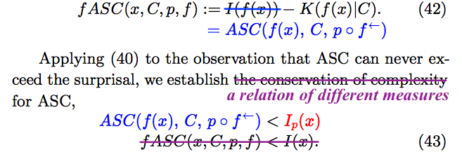
for all nonempty strings $x,$ Nemati and Holloway write

(43) $f\!ASC(x, C, p, f) < I(x)$

for all strings $x.$ Inequality (43) is what the authors refer to as “conservation of complexity.” When deobfuscated, in the next section of this post, the inequality turns out to be precisely equivalent to

$ASC(f(x), C, q) - ASC(x, C, p) < K(x|C).$

What the authors have managed to bound is the difference in the ASC of $f(x),$ according to a measure with chance hypothesis $q,$ and the ASC of $x,$ according to a measure with chance hypothesis $p.$

Deobfuscating “conservation of complexity”

The first principle is that you must not fool yourself—and you are the easiest person to fool. So you have to be very careful about that. After you’ve not fooled yourself, it’s easy not to fool other scientists. You just have to be honest in a conventional way after that.

— Richard P. Feynman, “Cargo Cult Science“

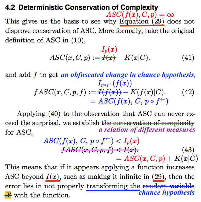
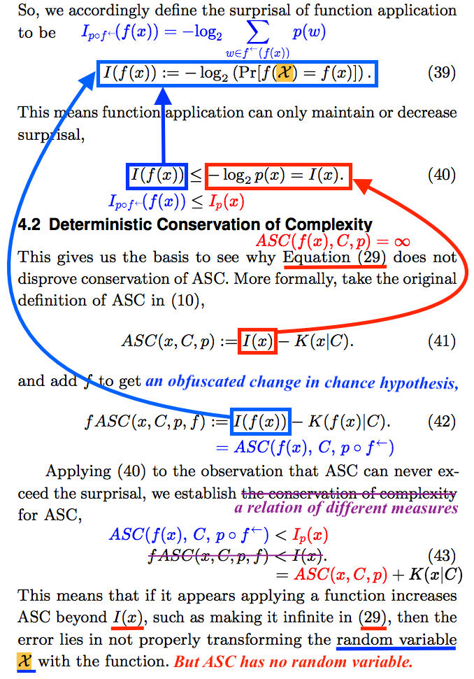
In “Stark Incompetence,” I provided general readers with a detailed parse of the mathematics in a passage like the one on display above. It is impossible to do the same here. Instead, I will break the passage into parts, and provide math-lite commentary. In broad overview, the authors have hidden, with egregious abuse of notation, a switch from one chance hypothesis to another. Most of my annotation of the passage is substitution of appropriate expressions for misleading ones.

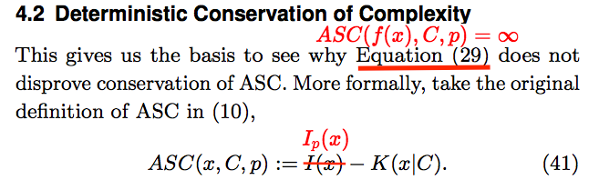
Section 4.2 begins with a remark that what comes at the end of the preceding subsection, addressed below, “gives us the basis to see why [infinite algorithmic specified complexity of $f(x)$ for all strings $x$ ] does not disprove conservation of ASC.” However, my proof of non-conservation identifies cases in which the ASC of the $x$ is finite and the ASC of $f(x),$ measured the same way as for $x,$ is infinite. The authors omit the crucial point that there is no upper bound on the difference in algorithmic specified complexity of $f(x)$ and $x$ that holds for all measures. They perhaps do this because their own expression of “conservation of ASC” does not make the difference explicit. We will find that there are hidden within the expression different measures of algorithmic specified complexity for the input data and the output data $x$ and $f(x).$

To reiterate an important point, algorithmic specified complexity is an infinite class of measures. The particular measure is determined by the settings of parameters referred to as the context and the chance hypothesis. The algorithmic specified complexity of data $x$ when the context is $C$ and the chance hypothesis is $p,$ denoted $ASC(x, C, p),$ is defined as the difference of two quantities, the first of which depends on the chance hypothesis, and the second of which depends on the context. It is easy to see, in the passage above, that the symbol $p$ does not appear in the ostensible definition of ASC. The authors should have written $I_p(x)$ instead of $I(x),$ making the dependence on the chance hypothesis explicit as they do elsewhere in the article. This is not nitpicking. In mathematical analysis, one should begin by making all details explicit, and later suppress details when there is no danger of confusion. Such discipline is a major aspect of how one avoids fooling the easiest person to fool.

As explained in the preceding section of this post, and as shown in the box above, $I_p(x)$ is the log improbability of the data $x.$ Although other investigators of algorithmic specified complexity refer to this term as the complexity of $x,$ Nemati and Holloway refer to it as the surprisal. As explained previously, $K(x|C)$ is the length of the shortest program that outputs the data on input of the context. Other investigators of algorithmic specified complexity have referred to $-K(x|C)$ as a measure of the specification of the data.

Now we examine the end of Section 4.1, which is referred to in the opening of Section 4.2. Recall that we corrected the definition of algorithmic specified complexity by making explicit the dependence of $I_p(x)$ on the chance hypothesis $p.$ Nemati and Holloway themselves use this notation elsewhere in the article, so there is no excuse for them not to have used it here. What they do instead is to engage in the most egregious abuse of notation that I ever have seen in a published paper. The authors make up a special rule for evaluating the expression $I(f(x)),$ the effect of which is to transform the chance hypothesis with the function $f.$ We write the frightening expression $p \circ f^\leftarrow$ for the transformed chance hypothesis, and replace instances of the inexplicit $I(f(x))$ with the explicit $I_{p \circ f^\leftarrow}(f(x)).$

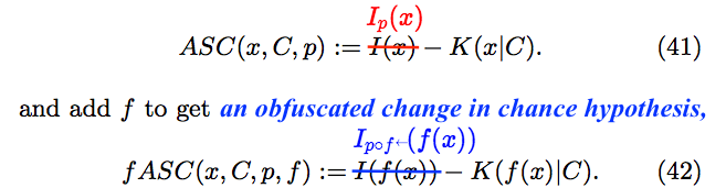
Now we pick up where we left off in Section 4.2. After repeating the definition of ASC, the authors define something new, called fASC. The very fact that they do this should send up a red flag. Why introduce fASC when addressing conservation of ASC? All readers should take a look at the annotation above. The authors have no good reason to repeat a definition that they gave earlier in the paper. What they do, by juxtaposing definitions in which the chance hypotheses are inexplicit, is to foster the false impression that the latter is obtained merely by replacing instances of $x$ in the former with the expression $f(x).$

Switching from inexplicit to explicit notation in Equation (42), we discover that fASC serves only to conceal a change in chance hypothesis. That is, fASC is just an obfuscated expression of the algorithmic specified complexity of $f(x),$ according to the ASC measure with context $C$ and chance hypothesis $p \circ f^\leftarrow.$

Eliminating fASC from what Nemati and Holloway call “conservation of complexity for ASC,” the result is a statement that the algorithmic specified complexity of $f(x),$ according to a measure with chance hypothesis $p \circ f^\leftarrow,$ is less than the log improbability $I_p(x)$ of $x$ under the chance hypothesis $p.$ This is very strange, because we naturally expect to see a comparison of two quantities of ASC in an expression of “conservation.”

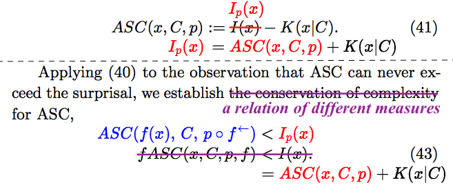
As shown at the top of the box, it takes just a bit of algebra to derive an expression of $I_p(x)$ in terms of algorithmic specified complexity. At the bottom of the box, $I_p(x)$ is rewritten accordingly. With just a bit more algebra, we find that (43) is tacitly an upper bound on a difference of the ASC of $f(x),$ according to a measure with $p \circ f^\leftarrow$ as the chance hypothesis, and the ASC of $x,$ according to a measure with $p$ as the chance hypothesis:

$ASC(f(x), \, C, \, p \circ f^\leftarrow) - ASC(x, \, C,\, p) < K(x|C).$

(I derive a tighter bound in the last section of this post.) As I said in the introduction, it would be absurd to speak to speak of (non-)conservation of a quantity of algorithmic specified complexity if different measures were applied to two strings. What Nemati and Holloway have derived is a relation of two different ASC measures. Their characterization of (43) as “conservation of complexity” is indeed absurd.

Wherefore art thou f(Montague)?

What’s in a name? that which we call a rose
By any other name would smell as sweet…

—William Shakespeare, Romeo and Juliet, 2.2

It is important to understand that a mathematical function $f$ defined on the set of all strings is not a computer program. The expression $f(x) = y$ indicates a particular relation of two strings. It does not indicate that something is done to one string in order to produce another. If we were to execute a program for calculation of $f,$ with $x$ as the input, then the output $y$ would be equal to $f(x).$ That would be “data processing.” But it should be clear that $y$ and $f(x)$ are two ways of denoting a particular string, and that the properties of the string do not depend on how we express it. Most importantly, the algorithmic specified complexity of the string does not depend on whether we refer to it as $f(x)$ or as $y.$ Furthermore, there are infinitely many computable functions $g$ for which $g(x)$ is the string $y,$ and in all cases the difference in ASC of $g(x)$ and $x$ is the difference in ASC of $y$ and $x.$

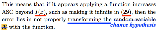
Now, if you get what I am saying, then you probably are wondering why I would bother to say it. The reason is that Nemati and Holloway do not get it. In the passage above, the authors characterize the expression $f(x)$ in my proof of non-conservation of ASC as “applying a function” to the string $x.$ What they have done is to introduce an alternative expression of algorithmic specified complexity, fASC, that treats the function $f$ as something that is done to $x.$ Simply put, they make the measure of algorithmic specified complexity of a string depend on how the string is expressed. In my proof, the string $f(x) = \lambda$ is infinite in algorithmic specified complexity. According to the authors, the string has infinite ASC when expressed as $\lambda,$ and “properly” has negative ASC, by a different measure, when expressed as $f(x).$

The authors make the strange claim that my “error lies in not properly transforming the random variable $\mathcal{X}$ with the function.” You need not know what a random variable is to understand my response. Two months before the authors submitted their paper for review, I told Holloway that there is no random variable in the definition of algorithmic specified complexity. As a matter of fact, the authors define ASC in Equation (10), and first write the symbol $\mathcal{X}$ in Equation (16) (15), without defining it. More precisely, what they define is $ASC(x, C, p),$ the algorithmic specified complexity of string $x$ when the context is $C$ and the chance hypothesis is $p.$ As explained above, $p(x)$ is the assumed probability of encountering string $x.$ Far into the article, the authors claim that the probability assigned to string $x$ by the chance hypothesis has been, all along, the probability that a random variable $\mathcal{X}$ has $x$ as its value:

So when we write $p(x)$ what we mean is

(34) $\begin{align*} p(x) & = \Pr[\mathcal{X} = x] \\ & \phantom{::} \vdots \\ \end{align*}$

Excuse me for laying a technical term on you, but people in my field refer to this as making shit up. You may think of $\mathcal{X}$ as a randomly arising string, and of the right-hand side of the equation as the probability that the string turns out to be $x.$ It follows from Equation (34) that the probability assigned to the string $f(x) = y$ by the chance hypothesis is the probability that the randomly arising string turns out to be $y$ :

$p(\underbrace{f(x)}_{=y}) = p(y) = \Pr[\mathcal{X} = y].$

The authors, who are on the losing end of a struggle with the rudiments of probability theory (I refer you again to “Stark Incompetence”), fail to see this. Evidently mistaking $f(x)$ as an expression of doing something to the string $x,$ they insist on doing the same thing to the randomly arising string $\mathcal{X}.$ That is, they believe that the probability assigned to $f(x)$ by the chance hypothesis ought to be the probability that $f(\mathcal{X})$ turns out to be $f(x):$

$\Pr[f(\mathcal{X}) = f(x)] \neq p(f(x)).$

What the authors refer to as “properly transforming the random variable $\mathcal{X}$ with the function” is replacing $\mathcal{X}$ with $f(\mathcal{X})$ when the string is referred to as $f(x)$ instead of $y.$

When the chance hypothesis is defined in terms of a random variable, a transformation of the random variable is necessarily a transformation of the chance hypothesis. Fortunately, and amusingly, with simplification of what ensues in the article, the random variable vanishes. The transformation of the chance hypothesis can be expressed, somewhat frighteningly, as $p \circ f^\leftarrow.$ It is much easier to explain the physical significance of the transformed chance hypothesis than to parse the expression. In essence, an unobserved process deterministically transforms a randomly arising string into an observed string. The transformation is modeled by the function $f.$ String $x$ enters unobserved into the process with probability $p(x).$ String $y$ is observed with probability $p \circ f^\leftarrow(y),$ which is equal to the sum of the probabilities $p(x)$ of all strings $x$ that the process transforms into $y.$

By way of explaining the context parameter of the measure $ASC(x, C, p),$ and also of driving home the point that $f(x) = y$ merely expresses a relation of strings, I turn to a pictorial example. The context $C$ can be any string, and here we take it to be an image-processing program that contains the Wikimedia Commons. Also, we adopt the chance hypothesis $p$ given by Ewert, Dembski, and Marks in “Measuring Meaningful Information in Images: Algorithmic Specified Complexity” (cited by Nemati and Holloway). That is, the log improbability of encountering an image is the number of bits in the image when it is converted to PNG format (and stripped of the header).

The Apotheosis of Meaning (at reduced resolution). The full-resolution image (3456 × 2592 pixels) contains 206 megabits of “meaningful information.”

The displayed image, which corresponds to a string $x,$ “looks random.” But there actually is nothing random about it. In particular, I did not sample the space of all images according to the chance hypothesis, i.e., with the probability $p(w)$ of drawing image $w,$ and then transform the image into $x.$ I wrote a short program that, on input of the context, outputs the image $x.$ (The program does this virtually: I have not constructed the context literally.) Referring to the function implemented by the program as $g,$ we can write $g(C) = x.$

As explained above, the algorithmic specified complexity of data $x$ is the difference in length of two recodings of the data. Here the data is an image, and the recoding associated with the chance hypothesis is the image in PNG format. The recoding associated with the context is the shortest program that outputs the image on input of the image-processing program containing the Wikimedia Commons. The length of the program that I used to transform the context into image $x$ is an upper bound on the length of the shortest program that does the trick. I do not know the precise length of my program, but I do know that it is less than 0.5 megabits. Thus, in my calculation that the algorithmic specified complexity $ASC(x, C, p)$ of image $x$ is approximately 206 megabits, I set $K(x|C)$ to 0.5 megabits. The string $x,$ representing the image titled The Apotheosis of Meaning, is an irreversible corruption of string $w,$ representing the following image from the Wikimedia Commons.

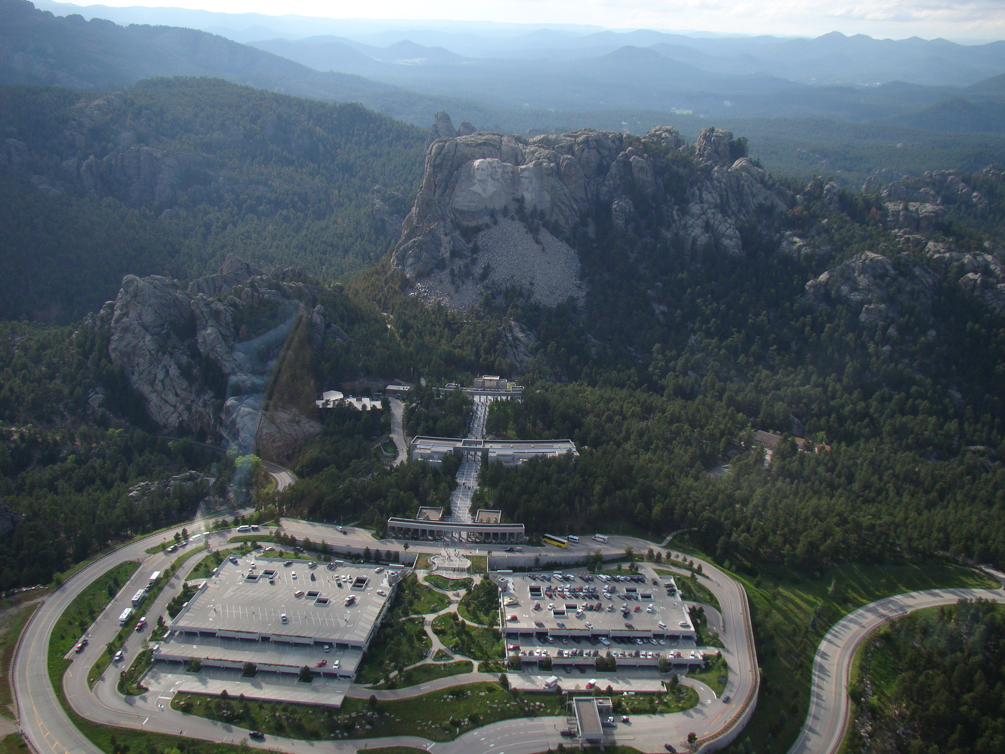
E.T. Views Rushmore (at reduced resolution). The full-resolution image (3456 × 2592 pixels) contains 102 megabits of “meaningful information.” Photo credit: Volkan Yuksel, via Wikimedia Commons (CC BY-SA 3.0).

The selection of an image of Mount Rushmore contained by the context $C$ is neither random nor arbitrary. My example is designed to embarrass Robert Marks (see why). The algorithmic specified complexity of $w$ is approximately 102 megabits, and the difference in ASC of $x$ and $w$ is approximately 104 megabits. Thus Marks, as well as his former students Nemati and Holloway, would have us believe that The Apotheosis of Meaning is twice as meaningful as E.T. Views Rushmore.

Recall that $g$ denotes the function computed by my program that transforms the context into the image $x,$ The Apotheosis of Meaning. That is, $g(C)$ is equal to $x$ . Nemati and Holloway presumably would not insist on changing the chance hypothesis to $p \circ g^\leftarrow$ when $x$ is referred to as $g(C).$ However, my program is easily modified to output $x$ on input of E.T. Views Rushmore, i.e., to compute a function $f$ for which $f(w)$ is equal to $x$ and $g(C).$ (The modified program cumulatively sums the RGB values in the input to produce the output, as explained in Evo-Info 4.) Now Nemati and Holloway object to my observation that the difference in algorithmic specified complexity of $f(w)$ and $w,$

$\begin{align*} ASC(\underbrace{f(w)}_{=g(C)}, C, p) - ASC(w, C, p) \approx 104 \times 10^6 \text{ bits}, \end{align*}$

is vastly greater than the length of a program for performing the “data processing” $f.$ They say that my “error lies in not properly transforming the random variable $\mathcal{X}$ with the function.” In other (and better) words, I should have changed the chance hypothesis to $p \circ f^\leftarrow$ in the measure of the algorithmic specified complexity of $f(w).$ But you know that I did not obtain $x$ by “applying a function” $f$ to a randomly selected string $w,$ as the transformed chance hypothesis would indicate. I have told you that I obtained $x$ by selecting a program, and running it with the context as input. You might say that I tacitly selected a function $g,$ and applied it to the context. You know that the expression $g(C) = x$ reflects how The Apotheosis of Meaning, represented by string $x,$ came to appear on this page because I have told you so, not because the expression itself tells you so. Similarly, the expression $f(w) = x$ indicates only a mathematical relation of $w$ to $x.$ It does not say that $x$ is the outcome of a process transforming $w$ into $x,$ let alone that $w$ is a random occurrence.

Supplement for the mathematically adept

Nemati and Holloway use the symbol $\mathcal{X}$ to denote both the set of all binary strings and a random variable taking binary strings as values. In the following, I write $\mathcal{X}$ for the set $\{0, 1\}^*,$ and $X$ for the random variable. I refer to elements of $\mathcal{X}$ as strings. The function $f$ is defined on the set of all strings, i.e., $f: \mathcal{X} \rightarrow \mathcal{X}.$

$ASC(x, C, p)$ is the algorithmic specified complexity of string $x$ when the context is $C$ and the chance hypothesis $p.$ The context is a string, and $K(x|C)$ is the algorithmic complexity of $x$ conditioned on $C$ (loosely, the length of the shortest computer program, itself a string, that outputs $x$ on input of $C$ ). There is actually another parameter here, the universal prefix machine in terms of which conditional algorithmic complexity is defined. But leaving it inexplicit is unproblematic. The chance hypothesis is a distribution of probability over $\mathcal{X}.$ The surprisal $I_p(x)$ is the base-2 logarithm of $1/p(x).$

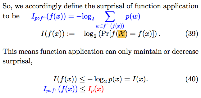
In the “definition” of fASC (42), the authors do not indicate that the probability distribution of the random variable $X$ in Equation (39) is the parameter $p.$ But their claims are correct only if we assume as much. In (39), the chance hypothesis, left inexplicit in the notation $I(f(x)),$ is the distribution of the random variable $f(X).$ In my expression $p \circ f^\leftarrow$ of the distribution of $f(X),$ I abuse notation slightly by writing $p$ in place of the corresponding probability measure $\mu_p$ on the space $(\mathcal{X}, \, 2^\mathcal{X})$ with $\mu_p(\{x\}) =$ $p(x)$ for all $x$ in $\mathcal{X}.$ I should explain also that $f^\leftarrow$ is a function from $\mathcal{X}$ to $2^\mathcal{X}$ with

$f^\leftarrow(y) = \{x \in \mathcal{X} \mid f(x) = y\},$

the set of all preimages of $y$ under the function $f.$ So for all $y$ in $\mathcal{X},$

$\begin{align*} p \circ f^\leftarrow(y) & = \mu_p(f^\leftarrow(y)) \\ & = \sum_{x \in f^\leftarrow(y)} \mu_p(\{x\}) \\ & = \sum_{x \in f^\leftarrow(y)} p(x) \\ & = \sum_{x : f(x) = y} p(x) \\ & = \sum_{x : f(x) = y} \Pr[X = y] \\ & = \Pr[f(X) = y]. \end{align*}$

I emphasize that there is no random variable in the definition of ASC. What the authors refer to as “properly transforming the random variable $\mathcal{X}$ with the function” is actually replacing the chance hypothesis with another. The new chance hypothesis essentially says that observed data result from unobserved processing $f(X)$ of randomly occurring data $X \sim p.$ That is, the $\mathcal{X}$ –valued random variable $X,$ modeling the unobserved input to $f,$ follows distribution $p,$ and $f(X),$ modeling the observed output, follows distribution $p \circ f^\leftarrow.$ It is important to understand that if I select $x$ and $f$ in order to make $ASC(f(x), C, p)$ large, and provide you with just the binary string $y = f(x),$ then your observation of large $ASC(y, C, p)$ gives you reason to reject $p$ as a model of how $y$ arose. If I tell you that I generated $y$ by applying function $f$ to $x,$ you do not have reason to replace the chance hypothesis with $p \circ f^\leftarrow,$ inasmuch as I did not obtain $x$ by sampling the distribution $p.$

Tightening the “conservation of ASC” bound

It is easy, and furthermore useful, to derive a “conservation of ASC” bound tighter than the one that Nemati and Holloway provide in (43):

$\begin{align*} & ASC(f(x), C, p \circ f^\leftarrow) - ASC(x, C, p) \\ & \quad = I_{p \circ f^\leftarrow}(f(x)) - K(f(x)|C) - [ I_{p}(x) - K(x|C)] \\ & \quad = I_{p \circ f^\leftarrow}(f(x)) - I_p(x) + K(x|C) - K(f(x)|C) \\ & \quad \leq K(x|C) - K(f(x)|C). \end{align*}$

The inequality in the last step follows from (40). If $x$ is the unique preimage of $f(x)$ under $f,$ i.e., $f^\leftarrow(f(x)) = \{x\},$ then (40) holds with equality, and the last line in the preceding derivation holds with equality. [Added equation to justify:]

$\begin{align*} I_{p \circ f^\leftarrow}(f(x)) & = -\!\log_2 \sum_{w \in f^\leftarrow(f(x))} p(x) \\ & = -\!\log_2 \sum_{w \in \{x\}} p(x) \\ & = -\!\log_2 p(x) \\ & = I_p(x). \end{align*}$

If, more restrictively, $x$ is the unique preimage of $\lambda$ under $f,$ then

$\begin{align*} & ASC(f(x), C, p \circ f^\leftarrow) - ASC(x, C, p) \\ & \quad = K(x|C) - K(f(x)|C) \\ & \quad = K(x|C) - K(\lambda|C) \\ & \quad = K(x|C) - O(1). \end{align*}$

Thus the difference of $A(f(x), C, p \circ f^\leftarrow)$ and $A(x, C, p)$ can be made large by selecting a string $x$ for which $K(x|C)$ is large, along with a function $f$ under which $x$ is the unique preimage of the empty string.

Improving upon the main result of the article

The following box contains what Nemati and Holloway describe as “the paper’s main result.” As indicated above, the symbol $\mathcal{X}$ is used to denote both a set and a random variable. Furthermore, $\mathcal{X}$ is not defined as a set or a random variable, either one. Again, I write $X$ for the random variable, and $\mathcal{X}$ for the set. In (15), the set $\mathcal{X}$ must be a subset of $\{0, 1\}^*,$ given the definition of $K(x|C).$ In fuller context, $\mathcal{X}$ is necessarily equal to $\{0, 1\}^*.$

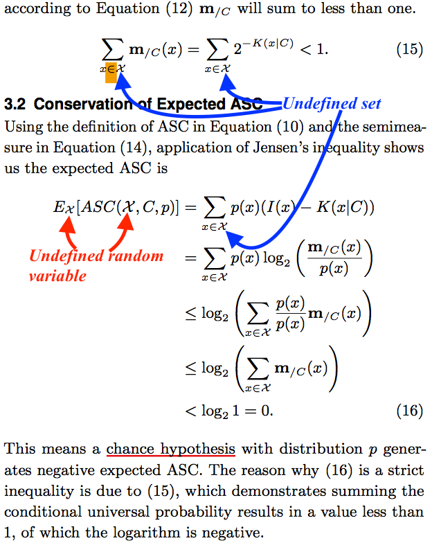
In the expression $E_\mathcal{X}[ASC(\mathcal{X}, C, p)],$ $\mathcal{X}$ must be a random variable. The only way to make the first equality in derivation (16) coherent is to assume that $p$ is a distribution of probability over $\mathcal{X},$ and that random variable $X$ follows distribution $p.$ The second line of the derivation would be the negative Kullback-Leibler divergence of $\mathbf{m}_{/C}$ from $p$ if $\mathbf{m}_{/C}$ were a proper distribution. To improve upon the result, turning the inequality into an equality, we need only normalize (regularize) the semimeasure $\mathbf{m}_{/C}$ to produce a probability distribution. Define probability distribution

$\mathbf{m}_{/C}^*(x) := \frac{ \mathbf{m}_{/C}(x) } { \mathbf{m}_{/C}(\mathcal{X}) }$

for all $x$ in $\mathcal{X} = \{0, 1\}^*,$ where

$\mathbf{m}_{/C}(\mathcal{X}) := \sum_{x \in \mathcal{X}} \mathbf{m}_{/C}(x).$

Writing $X$ for the random variable, and continuing from the second line of the derivation,

$\begin{align*} & E_X[ASC(X, C, p)] \\ & \quad = \sum_{x \in \mathcal{X}} p(x) \log_2 \left( \frac{\mathbf{m}_{/C}(x)}{p(x)} \right) \\ & \quad = \sum_{x \in \mathcal{X}} p(x) \log_2 \left( \frac{\mathbf{m}^*_{/C}(x) \, \mathbf{m}_{/C}(\mathcal{X})}{p(x)} \right) \\ & \quad = \sum_{x \in \mathcal{X}} p(x) \log_2 \left( \frac{\mathbf{m}^*_{/C}(x)}{p(x)} \right) + \sum_{x \in \mathcal{X}} p(x) \log_2 \mathbf{m}_{/C}(\mathcal{X})\\ & \quad = \sum_{x \in \mathcal{X}} p(x) \log_2 \mathbf{m}_{/C}(\mathcal{X}) - \sum_{x \in \mathcal{X}} p(x) \log_2 \left( \frac{p(x)}{\mathbf{m}^*_{/C}(x)} \right) \\ & \quad = \log_2 \mathbf{m}_{/C}(\mathcal{X}) \sum_{x \in \mathcal{X}} p(x) - D(p||\mathbf{m}^*_{/C}) \\ & \quad = \underbrace{\log_2 \mathbf{m}_{/C}(\mathcal{X})}_{< 0} - \underbrace{D(p||\mathbf{m}^*_{/C})}_{\geq 0}. \end{align*}$

The Kullback-Leibler divergence of $\mathbf{m}^*_{/C}$ from $p,$ $D(p||\mathbf{m}^*_{/C}),$ is zero if and only if the two probability distributions are identical.

Correcting some errors in Section 4.2

On display below is the passage that immediately follows the one on display above.

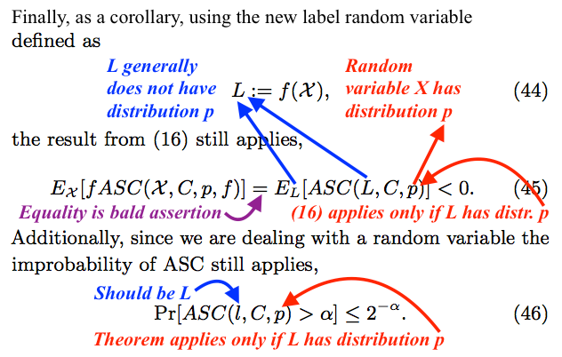
Again, we write $X$ for the random variable that Nemati and Holloway denote $\mathcal{X}.$ Recall that the distribution of $L = f(X)$ is $p \circ f^\leftarrow.$ When the inequality in (45) is revised to read

$E_L[ASC(L, \, C, \, p \circ f^\leftarrow)] < 0,$

it does follow from inequality (16). That is, as explained above, (16) is coherent only if the random variable is distributed according to the chance hypothesis. Furthermore, the equality in (45) holds because, as explained above,

$\begin{align*} f\!ASC(X, C, p, f) & = ASC(f(X), C, p \circ f^\leftarrow) \\ & = ASC(L, C, p \circ f^\leftarrow). \end{align*}$

Similarly, when (46) is revised to read

$\Pr[ASC(L, \,C, \,p \circ f^\leftarrow) \geq \alpha] \leq 2^{-\alpha},$

it follows from an emendation of Theorem 1 of Ewert, Marks, and Dembski, “On the Improbability of Algorithmic Specified Complexity”:

Theorem 1. The probability of obtaining an object exhibiting
$\alpha$ bits of ASC is less then [sic] or equal to $2^{-\alpha}.$

(2) $\Pr[ASC(X, C, P) \geq \alpha] \leq 2^{-\alpha}$

Interestingly, Ewert et al. also neglect to identify $X$ as a string-valued random variable following probability distribution $P.$ In the immediately preceding paragraphs of their paper, they identify $X$ as “the object or event or under consideration,” and also write $K(X|C),$ which indicates that the “object or event” actually must be an element of $\{0, 1\}^*.$ Thus it would seem that junk mathematics is being handed down from one Marks advisee to the next.

The most important of my annotations in the box above is the note that the equality in (45) is a bald assertion. If the authors had attempted a derivation, then they probably would have failed, and perhaps would have discovered how to correct their errors. I cannot imagine how they would have derived the equality without laying bare the fact that they modify the chance hypothesis. Note that with only $p$ written for the chance hypotheses in (45) and (46), there is nary a clue that that chance hypothesis is modified.

There are some similar errors in Sections 4.3 and 4.4. I will not spell them out. The authors should be able to find them, knowing now what they got wrong in Section 4.2, and address them in the errata that they submit to Bio-Complexity. I have spotted plenty of other errors. But life is short.

8 thoughts on “The old switcheroo”

J-Mac on January 30, 2020 at 5:32 pm said:

I have searched the OP carefully and found nowhere near any indications this applies to biology…
As I recollect correctly, EricHM has stated on more than one occasion that he doesn’t know whether his paper applies to real life… (biology/genetics).

If this is the case, why drag on this nonsense, if none of you is even willing to investigate the real life application?

Eric has a family of 5 to feed… Why would he even consider responding to this OP?
Neil Rickert on January 30, 2020 at 7:26 pm said:

J-Mac: I have searched the OP carefully and found nowhere near any indications this applies to biology…

That’s pretty much my reaction to all of the ID arguments about information.

Don’t blame Tom, as he is just responding to those arguments.
J-Mac on January 30, 2020 at 7:36 pm said:

Neil Rickert: That’s pretty much my reaction to all of the ID arguments about information.

Well, that’s just because of your ignorance…

Neil Rickert: Don’t blame Tom, as he is just responding to those arguments.

Read my, and Eric’s, comments again!
Do you need links???
EricMH on January 30, 2020 at 8:20 pm said:

I agree with J-Mac, very long, unclear article. Tom, can you provide a tl;dr that points out what my error is so I can respond to that?

Or better yet, submit a manuscript to Bio-C. Then it’ll get filtered for coherence. Once it’s passed that gate, then it’ll be clear to me it is worth my time to analyze and respond.
Tom English on January 30, 2020 at 8:49 pm said:

EricMH: I agree with J-Mac, very long, unclear article. Tom, can you provide a tl;dr that points out what my error is so I can respond to that?

Or better yet, submit a manuscript to Bio-C. Then it’ll get filtered for coherence. Once it’s passed that gate, then it’ll be clear to me it is worth my time to analyze and respond.

There’s a concise response in the last section, “Supplement for the Mathematically Adept.” Admittedly, I have argued that you are not a member of the target audience. Are you conceding the point?
Corneel on January 31, 2020 at 9:47 am said:

Thanks for taking the time to write this up, Tom. Nice to have the concept explained again.
Tom English on February 1, 2020 at 1:04 pm said:

From a comment of mine on “Questions for Eric Holloway”:

Eric Holloway has an ethical obligation to submit errata to Bio-Complexity when he is aware of errors in his article. Trying to shift the burden of submission to me is itself unethical.

You will find here a case in which some ID creationists, including the editor-in-chief of Bio-Complexity, attached an entire page of errata to a paper of theirs, in response to errors that I identified on my personal blog. They replaced five plots in the paper. (In fact, I diagnosed precisely the error they had made in processing the data that they plotted.) Interestingly, Eric Holloway recently referred to this paper. But rather than link to the freely available version containing the statement of errata, at the website of the Evolutionary Informatics Lab, he linked to a pay-to-view version without the errata. But surely that was merely an oversight on his part, for Eric is an honorable man.

I will point out, also, that Eric Holloway has benefitted from research that I have published on this blog. It was I, not any ID creationist, who discovered work by A. Milosavljecvic from 25 years ago that is quite similar to some published applications of algorithmic specified complexity. My discussion of Milosavljecvic comes toward the end of a long post, Evo-Info 4, that contains more math than does “The Old Switcheroo.” Eric Holloway happily benefits from that long post. But now, when a post identifies errors in an article of his, he claims that he does not have time to read it.
OMagain on February 1, 2020 at 1:25 pm said:

EricMH: Or better yet, submit a manuscript to Bio-C. Then it’ll get filtered for coherence.

Ever suggest that to gpuccio?

Does information theory support design in nature?