
Let us start by examining a part of the article that everyone can see is horrendous. When I supply proofs, in a future post, that other parts of the article are wrong, few of you will follow the details. But even the mathematically uninclined should understand, after reading what follows, that
- the authors of a grotesque mangling of lower-level mathematics are unlikely to get higher-level mathematics correct, and
- the reviewers and editors who approved the mangling are unlikely to have given the rest of the article adequate scrutiny.
Before proceeding, you must resolve not to panic at the sight of Greek letters and squiggly marks in the passage displayed below. Note that although the authors attempt to define a term, you need not know the meaning of the term to see that their “definition” is fubar. First, look over the passage (reading  as “zeta” and
  as “epsilon”), and get what you can from it. Then move on to my explanation of the errors. Finally, review the passage.
This is just the beginning of a tour de farce. I encourage readers who have studied random variables to read Section 4.1, and post comments on the errors that they find.
Everyone should see easily enough that the authors have not managed to decide whether the “countable set of events” is a discrete probability distribution  or a domain :
A discrete probability distribution
However, puzzling over the undefined term event may keep you from fully appreciating the bizarreness of what you are seeing. The authors in fact use the term to refer to elements of the domain. Here is an emendation of the passage, with event defined in terms of domain, instead of the reverse:
A discrete probability distribution
[The authors refer to individual elements of the domain as events, though an event is ordinarily taken to be a subset of the domain.]
Next, the authors attempt (and fail) to define as a set:
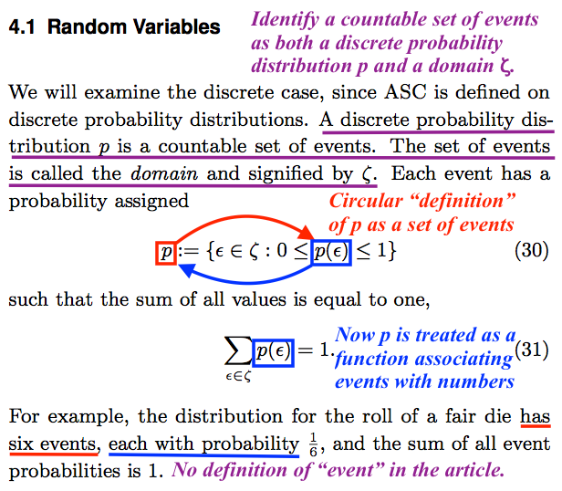
Each event has a probability assigned
(30)
![\[p := \{\epsilon \in \zeta :0\leq p(\epsilon) \leq 1 \} \]](http://theskepticalzone.com/wp/wp-content/ql-cache/quicklatex.com-0bf38a44ea8386e278aded433da0ada2_l3.png "Rendered by QuickLaTeX.com")
In plain language, Equation (30) says that is defined as the set of all elements of the set for which  is a number between
  and
and  The appearance of on both sides of the equation indicates that the authors have lapsed into circular definition — a fallacious attempt to define in terms of
  Furthermore, the authors use inconsistently. With the expression
 they indicate that is defined as the set of all events with a given property. However, their expression of the property,
  indicates that is not a set of events, but instead a function associating events with numbers. Equation (31) similarly treats as a function:
Each event has a probability assigned
(30)
such that the sum of all values is equal to one,
(31)
![\[\sum_{\epsilon \in \zeta} p(\epsilon) = 1. \]](http://theskepticalzone.com/wp/wp-content/ql-cache/quicklatex.com-e112906f45b111a8a52a699802abff4a_l3.png "Rendered by QuickLaTeX.com")
In plain language, Equation (31) says that the numbers associated with events in the domain sum to 1. Now, to gain an appreciation of how horribly confused the authors are, you should ponder the question of how they could use as a function in (31), associating events with numbers  and yet believe that they were correct in defining as a set of events in (30). In what immediately follows, the authors refer to the probability distribution as though it were both a set of events and a function associating events with numbers:
For example, the distribution for the roll of a fair die has six events, each with probability
and the sum of all event probabilities is 1.
What should the authors have written instead? The answer is not easy for general readers to understand, because I’ve written it as I would for mathematically literate readers. But here you have it:
A discrete probability distribution
of real numbers, with
For example, a roll of a fair die is modeled by distribution
for all
the set of all possible outcomes of the roll.
![\[\zeta = \{1, 2, 3, 4, 5, 6\},\]](http://theskepticalzone.com/wp/wp-content/ql-cache/quicklatex.com-8963120be664b24f4576d0124a43f5de_l3.png "Rendered by QuickLaTeX.com")
This says that for each of the elements of the set  the function associates with exactly one of the real numbers between 0 and 1. The number in the interval that is associated with is denoted
  I have omitted the term domain because the authors never use it. However, to plumb the depths of their incoherence, you need to know that the set is the domain of the function Here, to facilitate comparison with what I have written, is a repeat of the annotated passage:
Amusingly, the authors go on to provide examples of discrete probability distributions, in Equations (33) and (38), but misidentify the distributions as discrete random variables.
About one in ten of my sophomore students in computer science made errors like those on display above, so it would be unfair to sophomores to characterize the errors as sophomoric. I have never seen anything so ridiculous in the work of a graduate student, and have never before seen anything so ridiculous in a journal article. It bears mention that Nemati and Holloway were contemporaneous advisees of Robert Marks, the editor-in-chief of Bio-Complexity, as graduate students at Baylor University. Indeed, most of the articles published in Bio-Complexity have former advisees of Marks as authors.
[12/11/2019: Replaced a reference to (31) with a reference to (30).]
They thank you at the end of the article for “critical feedback”! I wonder if they’ll thank you for this bit of feedback
Could you explain how what they’ve done here can be used down the road to make a case for ID? ..because thats what this must be ultimately leading to…some attempt at a rigorous argument that complex systems cant evolve with a designer.
Obviously, they were trying to give a simplified definition, to make it easy to understand.
They simplified it so much, that it is nonsense.
Hahaha, good one!
Just for a hoot you should submit this to BIO-Complexity to see if they publish it, or see if they respond at all. 🙂
Section 4 does spend inordinate time reviewing math definitions that could just be cited from any textbook. As you point out, it then makes a hash of this unneeded review.
In any event, and perhaps unfairly, I suspect that the journal’s readership sees most of that mathematical review as “squiggly lines”.
Having spent some time with Section 3, it also seems to me that Sections 3 and 4 have nothing to do with each other.
For section 3, I’m still unclear on how distributions p and q fit into the numerical calculations; has anyone spent some time on working that out?
What they actually do is not to cite the post of mine that they’re drawing from, “Evo-Info 4: Non-Conservation of Algorithmic Specified Complexity.”
It’s hard to say, because IDists presently are going in two different directions with algorithmic specified complexity (ASC). Amusingly, Nemati and Holloway go both ways in a single article. In Section 2, they express their deep feeling that ASC is a measure of meaningful information. (Their conviction is so strong that they have no need to survey, or even mention the existence of, a large literature on meaningful / semantic information.) In Section 3, they treat ASC (actually, mean ASC) as a statistic. They measure high ASC on strings of bits generated by repeatedly sampling a Bernoulli distribution (e.g., repeatedly spinning a coin on its edge, with one side more likely to come up than the other, due to slight differences in the two sides). Nobody in his or her or its right mind would suggest that such strings are high in meaningful information. Thus Section 3 provides strong evidence that Section 2 is wrong in saying that ASC is a measure of meaningful information.
I’m sorry not to have answered the question you actually asked.
Little, but not nothing. A false inequality in Equation (45) of Section 4.2,
is contradicted by the results of Section 3.3. Let denote the distribution of random variable
  (Common shorthand:
  ) That is, for all binary strings
  the probability of
  is
is  An alternative expression of the inequality above is
In Section 3.2, “Conservation of Expected ASC,” the authors establish that this inequality holds in the case of In Section 4.2, it generally is not the case that distribution
  is identical to distribution
  and thus the inequality is unjustified. (In a forthcoming post, I will prove that the inequality is false.)
See what I wrote to RodW (thinking also, as I wrote it, of how I would respond to you). The authors obtain length-1000 binary strings by sampling the
  distribution. In simple terms,
  is the true distribution, and
  is the hypothesized distribution.
The authors approximate![E_q[ASC(L, C, p)],](http://theskepticalzone.com/wp/wp-content/ql-cache/quicklatex.com-69cd237946a51a4a42fe2c75c0de936c_l3.png "Rendered by QuickLaTeX.com") with
with  by taking the mean value of (an approximation of)
  for 100 samples
  of the
  distribution. They report positive approximate values of
 ![E_q[ASC(L, C, p)]](http://theskepticalzone.com/wp/wp-content/ql-cache/quicklatex.com-82ada1b4f527f03177bd5814607fd8f7_l3.png "Rendered by QuickLaTeX.com") when
when  diverges from
  Thus Section 3.3 contradicts a claim in Section 4.2. [ETA: They also formally derive positive expected ASC, but the result that they derive actually is not a precise match for the numerical experiment.]
Verily I say unto you, the left hand knoweth not what the right hand is doing in the article.
Has there ever been an article by Drs. Dembski, Marks and friends without miscalculations, botched simulations or at least an odd number of Vorzeichenfehler?
This one seems to be an egregious example, though: Kudos for wading through the swamp!
I doubt that I’ll ever learn to pronounce it correctly, but it certainly does have a lot more heft than sign error.
I’m not done with Nemati and Holloway yet.
Yes, I think I understood that was their purpose, but I wanted to make sure I understood the details in steps 1-4 where they are using compression as the way to calculate OASC to do that. In particular, step 3.
When they say they are using the LZW trained by the dictionary to compress the a string in step 3, I understand them to be saying that they have compressed the string by using LZW so that it in effect uses a dictionary which has been pre-built to compress most effectively strings generated according to q.
Given I am right on that, suppose the particular string generated is s and the training bitstring was t.
Is it correct to say they calculate OASC for a given s as follows:
log p(s) – I(s|t)
where I(s|t) is the approximate conditional KC calculated by the LZW compression..
I think their work is comparable to what Milosavljevic, 1995 does starting with Theorem 1.t
Using that theorem, Milosavljevic goes onto to show how to pick the null hypothesis distribution p. The null is that the strings are unrelated beyond the usual DNA chemistry; the alternative is that have have some common history. He si working with two fixed strings; and null hypothesis is the theoretical case where the smallest theoretically possible unconditional KC is obtained. The alternative has conditioning on the second string. He then goes on to derive a KMI in that case to do a hypothesis test of their relationship.
The equation in Milosavljevic Theorem 1 is ASC, I believe. But Eric’s joint paper is not generalizing the test in the same way. Rather than varying p to be the most challenging null hypothesis for fixed strings, they allow the distributions to vary [ETA] and then take a mean over many samples strings from q distribution.
Does that make any sense, even approximately?
ETA: Re-checking Milosavljevic, I see I reversed s and t from his Theorem 1. I had in mind sample string and training string for the above.
The million-bit string used to initialize the dictionary serves as the context C. The length of x, when compressed starting with the dictionary for C, is an upper bound on K(x|C).
In their analysis (part 2, in the right column of the same page), they derive the value of![E_q[K(\mathcal{X})]](http://theskepticalzone.com/wp/wp-content/ql-cache/quicklatex.com-ab0a216bd2dc038443ae02e4d0ac3836_l3.png "Rendered by QuickLaTeX.com") for
for  That is, they drop the context C in the analysis, and thus the analysis does not jibe entirely with the numerical experiment.
Yes. So you understand that this quantity has nothing to do with meaning — right?
I cannot recall what Theorem 1 was, and I’m not looking it up right now. Milosavljevic used a custom encoding scheme in his application, so his approach was more like that of Ewert, Dembski and Marks in, say, “Algorithmic Specified Complexity in the Game of Life” than that of Nemati and Holloway.
I think I understand you now. You have to keep it in mind that Milosavljevic is approximating algorithmic mutual information
I(x : y) = K(x) – K(x|y*),
where y* is a shortest program outputting binary string y. I can’t recall how he approximated K(x). But he could have done it by encoding the DNA sequence x as a binary string [ETA: straightforwardly, 2 bits per base], and then using LZW to compress it. The length of compressed-x is an upper bound on K(x).
ASC is, loosely, a generalization of algorithmic mutual information (AMI) because in AMI is replaced by
  in ASC, with
  an arbitrary distribution of probability over the set of all binary strings.
In considering work by Dembski, Marks, Ewert, and Holloway, there seem to be two approaches. One is to go through finding errors, one by one. The other is to try to figure out what the basic approach is, and what the objective is, and see whether the argument can be fixed. This is sometimes called setting up a “steel man” (by analogy to its opposite, a straw man). I have generally found that problems in their work can be fixed. But in some cases when we come to try to apply their argument to models of biological evolution, there are parts of the application that are just not explained. For example, in Dembski’s Law of Conservation of Complex Specified Information (2002), the sketched proof would be correct and devastating if the set of genotypes which is the target T could be kept the same (say, all the highest-fitness genotypes). But the proof sketched in No Free Lunch changes that set from one generation to another. And there is no discussion of which of those is appropriate to do, and even whether the objective is to show that fitness cannot increase in a run of a genetic algorithm.
That’s true with Holloway’s argument too. Even if any glitches can be fixed (in the present case maybe they can’t), what is the rest of the argument? So far, there is silence on that.
As best I can tell, Eric is making two arguments in his posts over the last year at TSZ.
The first is based on Levin’s conservation of KMI and was made last December. That argument is fine mathematically. But the mathematics needs a biological model to have any relevance to evolution via NS. As you point out at PT, even a simple model would do, as long as it captures all relevant aspects of NS. So the issue here is to isolate the relevant aspects of NS, eg populations and selection by fitness in an environment with state and dynamics consistent with physics. Eric has not done that.
Eric’s second, current argument is based on the purported conservation of ASC. But the math regarding conservation of ASC in the paper under discussion is far from acceptable. So there is no reason to even ask for a biological model. If the math did work, then a model that worked for Levin’s KMI result would do (or so Eric claims at PT).
Right, I think I understand that and I think I understand the details of why AMI is a special case of ASC. My point is that Milosavljevic, 1995 and the paper both start with an ASC formalism but then moving in different directions because they have different entities they want to vary in their tests.
But it’s just to help me verify the correctness of my understanding of ASC, AMI, and section 3. So I am happy to leave it and concentrate on the paper.
Yes, that was what I was trying to say, so you’ve confirmed what I was thinking, if not expressing well.
Now I read the expectation in 16 is taken with respect to a fixed p. That is, it is not the expectation over varying contexts, which would mean somehow taking an expectation with respect to q if I understand your above quoted text correctly.
I have more to say on the resulting relation to section 4, but I want to make sure that what I said so far makes sense.
I also want to be clear that I think you have raised substantive concerns with the math of Eric’s arguments in section 4, and as I posted earlier in the Addendum thread, I think Eric should have addressed those issues rather than passing the buck to whoever referees BIO-C. But I am putting those concerns aside for the sake of argument in discussing 3 versus 4.
It is awful. I was not well at the time Eric posted it. Otherwise, I would have said much more.
The opening post of this thread illustrates how bad Eric is at basic definitions. Most people can understand most of the OP. Eric also mangles algorithmic information theory. However, relatively few people understand AIT, and Eric expresses great confidence in himself. So folks mistakenly assume that he probably knows what he’s talking about.
Eric doesn’t even get ID right. The stuff he says about Dembski’s earlier work is bizarre.
I am a long-time critic of ID. Never before have I characterized the stuff coming from a credentialed ID proponent as crankery. But I’m doing it now. Jeffrey Shallit was saying much the same seven years ago:
Eric had only a master’s degree in computer science at the time. He now has a doctoral degree in electrical and computer engineering. So what!? He should not have been saying such ridiculous stuff with a master’s degree. An additional 2.5 years of schooling at Baylor University did not change him into a different kind of person. How anyone could look at what I’ve detailed in the OP, and doubt that it “would be laughed out of any real scientific or mathematics” venue, is beyond me.
We worked together on understanding the last paper on conservation of active information. There was something rigorous enough there to be grasped and addressed.
The problem here is that you have asked Eric Holloway what conservation of ASC has to do with biological evolution. You definitely mean
where and
and  are binary strings, and
  is a distribution of probability over the binary strings. But when Eric replies, is he talking about ASC?
In Section 3.2, “Conservation of Expected ASC,” there is a correct result. But Eric was never talking about expected ASC in the sources that you linked to in your PT post. What he was saying last year was that the conservation (non-growth) of algorithmic mutual information result extended to ASC. He has yet to acknowledge that he was wrong, but he has acknowledged that one of my proofs of the contrary is right.
What Nemati and Holloway call “the conservation of complexity for ASC” in Section 4.2 is actually a result for fASC,
So if Eric addresses your question as to what conservation of ASC has to do with biological evolution, has he changed from ASC to (the very different) fASC, without telling you what he’s done?
Then again, the bound![\Pr[ASC(X, C, p) \geq \alpha] \leq 2^{-\alpha}](http://theskepticalzone.com/wp/wp-content/ql-cache/quicklatex.com-48cd1178e8f907e7244013c507c1cfd9_l3.png "Rendered by QuickLaTeX.com") also appears in the article by Nemati and Holloway. George Montañez calls this bound conservation of information, but Nemati and Holloway do not. But perhaps Eric will start referring to it as conservation of ASC, and referring to the bound in his article as conservation of fASC.
also appears in the article by Nemati and Holloway. George Montañez calls this bound conservation of information, but Nemati and Holloway do not. But perhaps Eric will start referring to it as conservation of ASC, and referring to the bound in his article as conservation of fASC.
What I’m driving at is that you must get Eric to commit to formal definitions of terms.
There’s another post coming. It will address Section 4. Please save what you have.
Correct. The first step in the derivation expresses the expectation in terms of p, so the result is most definitely predicated on
The rest of the argument is the standard ID argument put forward by Dembski: if we have something that can be described concisely with an independent context, but is improbable in light of natural processes, then the source of the alternate context is the better explanation. So, if the context is defined in terms of intelligent agents (i.e. humans), then that indicates intelligent agency is a better explanation of the event in question than natural processes.
Side note, while fitness could perhaps be a specification in Dembski’s argument, it is not obviously so, and that’s why Dr. Felsenstein’s question about fitness defined specifications, while interesting and I intend to respond using algorithmic information, is not directly relevant for Dembski’s argument.
There’s been some controversy regarding whether processing events (e.g. with evolutionary algorithms ) can somehow make these unlikely events more likely, and thus create information, and that’s what our paper addresses. The answer is ‘No’, at least in terms of taking the expectation over the relevant random variable(s). I also like how the expectation is a strict bound instead of a probabilistic bound, but I don’t know if that is significant.
We talk about ‘meaning’ because ASC measures whether an event refers to an independent context, i.e. measures whether X ‘means’ Y, like a signpost.
And yes, Dr. English made the good point that ASC is problematic in this regard since I(X) – K(X) might equal I(X) – K(X|C), in which case high ASC doesn’t necessarily indicate X refers to C. But, that is not an irredeemable flaw, and it’s a separate issue from the conservation bounds proven in our paper.
Finally, I’m very interested in whether Dr. English can discredit a ‘steelman’ version of our paper. I’m sure he can find plenty of flaws, but as usual they are not essential to the argument, so at least do not provide any useful information to me whether there is something fundamentally flawed about the ID argument. Of course, by pointing out my mistakes Dr. English can make a decent go at poisoning the well, and making people doubt the merits of the paper by doubting my competence. He certainly makes me feel ashamed of my sloppy work, regret not being more careful, and doubt whether I even deserve a PhD. And that’s great as far as PR goes. But, it is ultimately not valuable as far as the truth of the matter is concerned. I’m certain that Dr. English is much more competent than myself, and can see through the horrible mathematics to the heart of the proof, and say whether the logic ultimately holds or not.
How did you determine natural evolutionary processes and their results are improbable?
You use an awful lot of verbose bluster to say “God of the gaps”.
If you’ve read any of my responses to this claim, repeated often on this forum, and carefully thought through them, you’d know that is not the case.
Anyways, I await Dr. English’s disproof of the ‘steelman’ version of our paper, and otherwise I probably will not comment further.
You dodged the question.
How did you determine natural evolutionary processes and their results are improbable?
Alright, one more response then, you need to understand the terms being used here. Natural processes are said to be probabilistic in some regard, so we can talk about the probability of their outcomes. That is all I’m referring to. I am not making any concrete argument about any specific biological entity and its likelihood of occurrence due to evolution. I am only talking about the mathematics behind such arguments, as it is the only area I am qualified to make some sort of statement. I’m not qualified to say anything about biology or evolution itself, except insofar as it can be modeled by mathematical and computational processes.
And now I’ll await Dr. English’s disproof of the steelman version.
So far your attempts at modeling actual evolution have been piss poor to non-existent, yet that hasn’t stopped you from making some rather ridiculous claims about evolution’s impossibility. Why is that?
If you actually wanted me to respond to a “steelman version,” then you would tell me now what that “steelman version” is. Otherwise, you are merely waiting to tell yet another story of something that you established in the paper, even though it is not to be found in the paper.
Thank you for making an effort to address this. It is a refreshing change from the responses I have seen so far.
So there is some assertion (by who?) that living organisms can be described very simply. Their genotypes? Their phenotypes? That has never been explained. And ordinary evolutionary processes such as natural selection cannot achieve that simple a description? I see no proof of that, or attempt to prove that. Of course, it is not obvious why natural selection should favor simplicity of description as opposed to favoring increase of fitness.
I have many times quoted this passage, from page 148 of Dembski’s No Free Lunch: Why Specified Complexity Cannot Be Purchased without Intelligence:
Note: not simplicity-of-description, but in each case components of fitness or measures of fitness. That includes “function of biochemical systems” which are only worthwhile if they contribute to fitness.
Leaving aside the issue of whether those bounds are proven (which others here have investigated), when we forget about simplicity of description and ask about the kinds of specification that Dembski described, the whole attempt to show conservation-of-simplicity-of-description is simply a mathematically-complex digression that does not show anything that puts a constraint on what evolution can do in the way of achieving adaptation.
As far as I can see the whole attempt to find laws of conservation started with CSI, and was thus basically an attempt to argue that natural selection could not increase fitness substantially. That it would not work to achieve adaptation.
Evolutionary algorithms work in terms of fitness, not simplicity-of-description. They do show that fitness can increase in those models as a result of selection. The issue of whether they get the genotype’s bitstring close to, say, the binary encoding of is of no biological interest.
The rest of Eric’s response is addressed to Tom, so I break off here.
(see my next comment)
I’ve emailed a copy of this comment to Eric Holloway. I used the address given at the top of his article. I tried repeatedly to send a TSZ message to EricMH, but never got things to work.
ETA: Email bounced back to me from Baylor.
At Panda’s Thumb, in a comment he made (self-identified as user “yters”) on
the ASC thread, Eric pointed us to a 2018 comment at TSZ where he argued that if Y was a bitstring which was the “target”, and X a bitstring that was the genotype, then adding a bitstring R of random bits would not help X have more mutual information with Y. And that this was what the conservation result could show.
Basically in such a case, we have a Weasel model with an individual, a new string R, and selection favoring whichever is closer to the target. I suggested, a little later in that thread, that we replace R by a mutated copy of the parent. If the mutation got R closer to Y than X was, it would replace X. Such a model will show X to converge on Y. Mutual information about the target, which reflects the environment, is gradually and cumulatively built in to X. Is information “created”? Or is it arriving from changes in entropy in the system? We don’t need to answer that to see that any conservation result for mutual information does not stop the change of mutual information in that model.
Thanks to EricMH for, in the passage cited in that thread, getting the model so close to being a Weasel. In the binary Weasel with a target (given by the environment) and selection between a genotype and its mutated offspring, the selection between two alternatives is what makes the process move toward the target.
Note: The links above to comments in the PT thread works best if you open up all comments in that thread so the link can find them.
Joe Felsenstein,
I butted out of your thread at PT, and let yters lie about me, just so you could do your thing with him (or her or it). What you’re repeating here is crankery. I am not, in this thread, going to deconstruct what EricMH posted a year ago, on another topic. So I ask that you not use this thread to aid EricMH in propagating what I regard as crankery.
The PT commenter yters claimed that he (or she or it) was going to respond to a request of yours by posting here at TSZ. So, if you believe that EricMH is yters, hold him to making a new post. Please do not pursue the matter here.
Tom English,
I will respect your request. yters self-identified, in earlier comments at PT, as Eric Holloway. My comments here do not accept Eric’s assertions about conservation, but argue that even if conservation were true, that is not sufficient. Anyway I will put up a new post at PT so he can discuss this with me there.
Joe Felsenstein,
As you know, if a putative model is logically inconsistent, then it is not a model of anything. I claim that that EricMH’s putative model is logically inconsistent. You had better prove that it is consistent, or turn it into something that you can prove is consistent, before going on to discuss its biological relevance.
[Edited: removed some “logically” instances.]
I meant Levin’s “conservation” result is fine mathematically. I do that in order to contrast the general acceptance of the math of this result with the outstanding math concerns with the arguments on conservation of ASC in section 4.
As I said to Joe, I think Eric is making two arguments: one last year based on Levin’s work where he tries to relate it to biology, and one this year where he tries to develop an analogous conservation result for ACS.
I am not saying that Eric argues well or succesfully in either case. I am only trying to express what I see him as doing charitably. For me, doing that is an important part of any useful exchange of views.
Do you agree with my understanding that Eric is making two arguments?
ETA: I see Eric has replied to Joe’s concerns about Dembski. That’s a third argument, not directly related to the December 2018 posts or the conservation of ACS posts.
I see you’ve told Joe you are not interested in the Dec 2018 posts. Fair enough: I will stop mentioning them.
I am not sure Eric understands “steelman”: one does not steelman one’s own arguments, AFAIK.
Belly laugh!
I seem to be typing ACS instead of ASC in some of my notes. Oops.
Re: “steelman”, you have presented counterexamples to Eric’s assertions. Therefore there is no way to make a steelman argument for his assertions except by changing what the assertions are, to ones that are similar (in some relevant sense) but can actually be proven.
I am saying “even if”. Even if EricMH were right about conservation of ASC, he would still have the burden of showing that this placed some constraint on evolution. And he has not shown that. (I will, as you requested, continue that discussion with a new post at PT, and not here).
I apologize for being short with you. To make amends, I will post a brief OP today. I’ll identify a preliminary hurdle that must be cleared before Holloway has any chance at all of making consistent claims. This has nothing to do with conservation of information.
Apologies for this. I checked, and while the text in the URL is correct, if you instead click on it and have it automatically populate the email, it’ll use the incorrect ‘Holloway@baylor.edu’.
I intend to submit a corrected article, including notational corrections as you point out in the OP, and anything else that turns up.
By ‘steelman’ version I mean there is an actual argument I am making in the paper, which your deconstruction of my notation, while valid, does not address at all. I believe, despite my incorrect notation, you are able to understand my argument and address it, along with any logical flaws you identify.
This, I assume, is your refutation of my core argument. And I can see it is my fault due to the incorrect notation I used.
But, you are comparing apples and oranges by referring to 3.3 as a contradiction of 4.2. 3.3 deals with different distributions over the same set of events. 4.2 deals with potentially different sets of events.
Again, it is probably my bad notation that is causing this confusion, or perhaps you are not reading the paper carefully enough, but once the confusion is cleared up, the math holds without problem.
It indeed is. I should have used the distribution p_L instead of p in that particular equation. As it stands, the equation is incorrect, as Dr. English points out.
Thanks for taking the time to try to address Tom’s concerns directly and succinctly and also for concentrating on the math.
No, I tried using the text, and several obvious variations, and never got a message through to you.
You have, with the most egregious abuse of notation I have ever seen in a peer-reviewed publication, concealed a huge flaw. It is highly inappropriate for you to deflect with “just notation” remarks. It took me much longer than it should have to see the absurdity of your “conservation of complexity for ASC” claim, because I fixated on the errors downstream, and got locked into thinking about things the wrong way. This ultimately was your fault, not mine. You have wasted a lot of time of a reader who always has striven not only to get at what you intend to say, but also to understand your misunderstandings.
The most generous assumption is that you in fact do not know what you actually are saying, when you write
(43)![\[f\!ASC(x, C, p, f) < I(x), \]](http://theskepticalzone.com/wp/wp-content/ql-cache/quicklatex.com-66327bde0fb324477d75493897cf337e_l3.png "Rendered by QuickLaTeX.com")
and refer to the inequality as “conservation of complexity for ASC.” Otherwise, you are guilty of intentionally withholding from readers the fact that you apply different ASC measures to the input and the output
  and furthermore misleading them by attributing to me the error of “not properly transforming the random variable
  with the function.” That is to say, you have fooled yourself by using inexplicit and misleading notation.
Your “it’s just the notation, not the logic” tactic is not going to work. If you truly do know already that Equation (43) conceals a change from one ASC measure, for the input to another ASC measure, for the output
  and have not explained as much, then you are a sorry excuse for a human being. But I know from what comes earlier in Section 4, including the passage on display in the opening post of this thread, that you understand the math poorly.
It may be, now that I’ve given you an expression of the chance hypothesis in the ASC measure that you apply to
  that you can rewrite (43), and make the change in chance hypothesis explicit. But if you claim to have known all along that (43) conceals a change in chance hypothesis, then you will be guilty either of lying now or of intentionally misleading readers when you wrote your paper. I sincerely hope that what you will do instead is to acknowledge that you have learned the hard way how important it is, in mathematical analysis, to use appropriate notation.
ETA: In the other thread, I mentioned slight abuse of notation in I’ve written
  in place of the corresponding probability measure
  on the space
  with
with  for all
  in
in 
I will have to see you unpack this claim. As far as I know, I made it clear how the chance hypothesis is modified through function application in section 4.1.